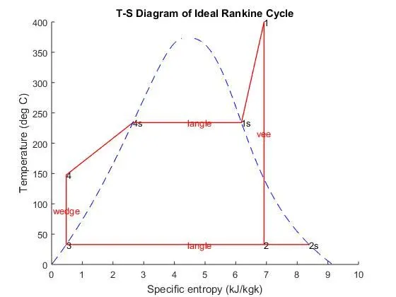
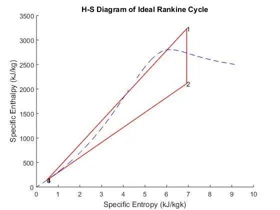
Project 2 - Rankine cycle Simulator

AIM: Writing a code to simulate Rankine Cycle.

OBJECTIVE: -

• Create a Rankine cycle simulator using MATLAB.
• Your code should calculate the state points of the Rankine cycle (any type of choice) based on user inputs.
• Then, plot the corresponding T-S and H-S plots for the given set of inputs. Title and axes labels are a must, while legends could be used if necessary.
• The presentation of your code using comments is appreciated.
• Attach a report explaining the working of a Rankine cycle simulator and also the research done by you.

THEORY: -

The Rankine cycle is a model used to predict the performance of steam turbine systems. Rankine cycle consists of an operating fluid that continuously gets evaporated and condensed in a close loop.

1. Boiler for generating steam at constant pressure.
2. A turbine or engine in which steam will expand isentropically and work is done.
3. A condenser in which heat is removed from the exhaust steam and is completely converted into the water at constant pressure.
4. A pump that raises the pressure of liquid water to boiler pressure and pumps it into the boiler for converting into steam.

Basic Rankine Cycle Simulator

Process:

1-2: Isentropic compression in pump

2-3: Constant pressure heat addition in the boiler

3:4: Isentropic expansion in the turbine

4-1: Constant pressure heat rejection in the condenser

Code:

clear all
close all
clc

disp(' SIMULATOR OF RANKINE CYCLE ')
disp('1-2 Isentropic Expansion in the Turbine ')
disp('2-3 Constant Pressure Heat Rejection by the Condenser ')
disp('3-4 Isentropic Compression in the Turbine ')
disp('2-3 Constant Pressure Heat Addition by the Boiler ')

% Inputs
disp('INPUTS');
p1 = input('Enter the Pressure at the Turbine Inlet (in bar): ');
T1 = input('Enter the Temperature at the Turbine Inlet (in Degree celsius): ');
p2 = input('Enter the Pressure at the Condenser (in bar): ');
disp('Results')

%getting Cp and Cv values from XSteam

% for Vapour
high_CpV =XSteam('CpV_p', p1);
low_CpV =XSteam('CpV_p', p2);
high_CvV =XSteam('CvV_p', p1);
low_CvV =XSteam('CvV_p', p2);

% for liquid
high_CpL =XSteam('CpL_p', p1);
low_CpL =XSteam('CpL_p', p2);
high_CvL =XSteam('CvL_p', p1);
low_CvL =XSteam('CvL_p', p2);

% Getting important parameters from XSteam

% for high pressure
T1s = XSteam('Tsat_p',p1);
s1g = XSteam('sV_p', p1);
s1f = XSteam('sL_p', p1);
s1fg = s1g - s1f;
h1f = XSteam('hL_p', p1);
h1g = XSteam('hV_p', p1);
h1fg = h1g - h1f;

% for low pressure
s2g = XSteam('sV_p', p2);
s2f = XSteam('sL_p', p2);
s2fg = s2g - s2f;
T2s = XSteam('Tsat_p', p2);
h2f = XSteam('hL_p', p2);
h2g = XSteam('hV_p', p2);
h2fg = h2g - h2f;

%% State point 1

disp('At State point 1:');

fprintf('p1 is: %f Barn\n', p1);

fprintf('T1 is : %f Deg celcius\n', T1);

h1 = XSteam('h_pT', p1, T1);
fprintf('h1 is: %f kJ/kg\n', h1);

s1 = XSteam('s_pT', p1, T1);
fprintf('s1 is : %f kJ/kgk\n', s1);

%% State point 2

disp('At State point 2:');

fprintf('p2 is: %f Barn\n', p2);

s2 = s1;
%predicting location of point 2 in T-s
if (s2<=s2g)
x2 = (s2 - s2f)/(s2fg);
else
x2 = 1;
end
fprintf('x2 is %f \n',x2);
% calculating T2 for superheat or wet or dry wherever it lies
if (x2<1)
T2 = T2s;
else
%t2 cal by s2=s2g+low_CpV*(log(T2/T2s))
T2 = ((T2s+273.15)*exp(s2-s2g)/(low_CpV));
T2 = T2-273.15;
end
fprintf('T2 is : %f Deg celsius \n',T2);

if (x2<1)
h2 = h2f + x2 * h2fg;
else
h2 = h2g + low_CpV*(T2-T2s);
end
fprintf('h2 is : %f kJ/kg\n', h2);

%% State point 3
% Assuming no subcooling in condensor
disp('At state point 3:');

p3 = p2;
fprintf('p3 is : %f Barn\n', p3);

v3 = XSteam('vL_p', p3);

T3 = T2s;
fprintf('T3 is : %f Deg celsius\n', T3);

h3 = h2f;
fprintf('h3 is : %f kJ/kg\n', h3);

s3 = s2f;
fprintf('s3 is : %f kJ/kgk\n', s3);

%% State point 4
disp('At state point 4:');

p4 = p1;
fprintf('p4 is : %f Barn\n', p4);

s4 = s3;
fprintf('s4 is : %f kJ/kgk\n', s4);

wp = v3 * (p4 - p3) * 100;
h4 = wp + h3;
fprintf('h4 is : %f kJ/kgk\n', h4);

% to cal T4 s4=s3=sf1-high_CpL*ln(t1s/t4)
term=exp((s1f-s4)/high_CpL);
T4 = T1s/term;
fprintf('T4 is : %f Deg celsius \n', T4);

%% Workdone, heat, SSC and efficiency calculations
wt = h1 - h2;
fprintf('Work by turbine is : %f kJ/kg\n', wt);
fprintf('Work by compressor is : %f kJ/kg\n', wp);
wnet = wt - wp;
fprintf('Net Work done is : %f kJ/kg\n', wnet);
Qin = h1 -h2;
eff_thermal = wnet /Qin; % Efficiency
fprintf('Thermal efficiency is : %f\n', eff_thermal); disp('%')
SSC = 3600/ wt; % Specific steam consuption
fprintf('.S.S.C is : % f kg/kwh\n', SSC);

%% Calculation for plotting Liquid and Vapour Lines
%
% <<FILENAME.PNG>>
%
temp = linspace(1, 373, 500);
for i = 1: length(temp)
H_L(i) = XSteam('hL_T', temp(i));
H_V(i) = XSteam('hV_T', temp(i));
S_L(i) = XSteam('sL_T', temp(i));
S_V(i) = XSteam('sV_T', temp(i));
end

%% Plotting T-S and H-S Diagrams

figure(1) %T-S
hold on
plot([s1 s2],[T1 T2],'r','linewidth',1)
text(s1,T1,'1')
text(s2,T2,'2')
plot([s2 s2g],[T2 T2s],'r','linewidth',1)
text(s2g,T2s,'2s')
plot([s2g s3],[T2s T3],'r','linewidth',1)
text(s3,T3,'3')
plot([s3 s4],[T3 T4],'r','linewidth',1)
text(s4,T4,'4')
plot([s4 s1f],[T4 T1s],'r','linewidth',1)
text(s1f,T1s,'4s')
plot([s1f s1g],[T1s T1s],'r','linewidth',1)
text(s1g,T1s,'1s')
plot([s1g s1],[T1s T1],'r','linewidth',1)
plot(S_L, temp, 'b','linestyle','--','linewidth',1)
plot(S_V, temp, 'b','linestyle','--','linewidth',1)

%marking direction
text(s1,(T1+T2)/2,'vee','HorizontalAlignment','center','color','r')
text(((s2g+s2f)/2),T3,'langle','color','r')
text(s3,(T3+T4)/2,'wedge','HorizontalAlignment','center','color','r')
text((s1f+s1g)/2,T1s,'langle','color','r')
title('T-S Diagram of Ideal Rankine Cycle')
ylabel('Temperature (deg C)')
xlabel('Specific entropy (kJ/kgk)')

figure(2) %H-S
hold on
plot([s1 s2],[h1 h2],'r','linewidth',1)
text(s1,h1,'1')
plot([s2 s3],[h2 h3],'r','linewidth',1)
text(s2,h2,'2')
plot([s3 s4],[h3 h4],'r','linewidth',1)
text(s3,h3,'3')
plot([s4 s1],[h4 h1],'r','linewidth',1)
text(s4,h4,'4')
plot(S_L, H_L, 'b','linestyle','--','linewidth',1)
plot(S_V, H_V, 'b','linestyle','--','linewidth',1)
title('H-S Diagram of Ideal Rankine Cycle')
ylabel('Specific Enthalpy (kJ/kg)')
xlabel('Specific Entropy (kJ/kgk)')

Explanation of Code: -

1. Clear all, close all, clc – to clear the command window and remove previous variables in the workspace.
2. fprintf – to print required lines in the command window.
3. input – to get values of input conditions from a user.
4. XSteam – custom function to get values from a steam table.
5. if-else – to calculate fractions
6. for – to create points to plot dry saturated liquid and vapour line.
7. plot – to plot the graph based on input.
8. text – give a name to points in the plot.

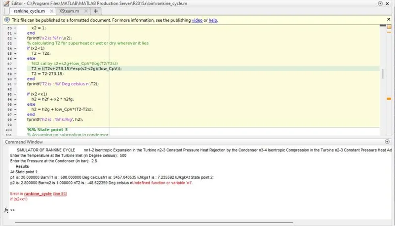
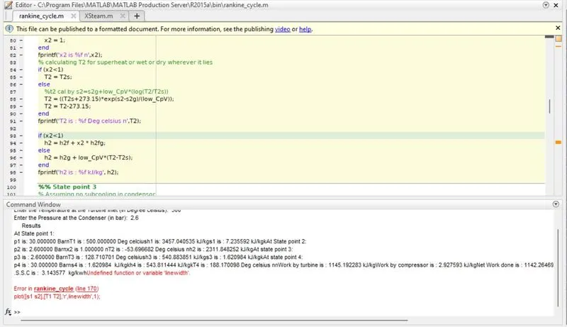
Errors:-

Errors occurred during the program.

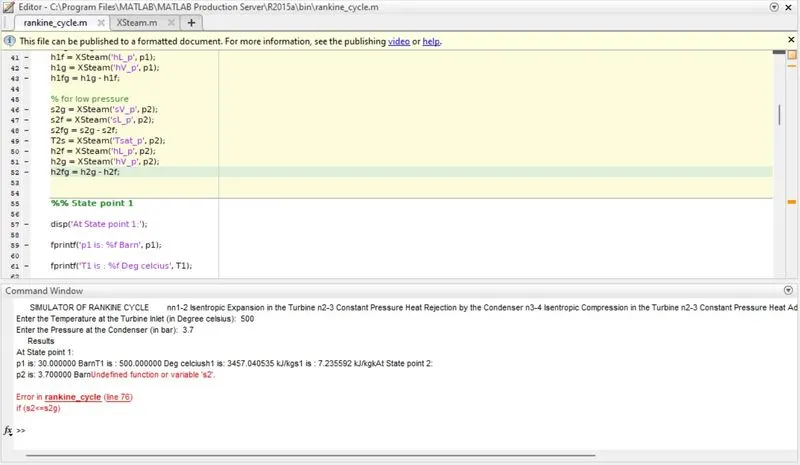
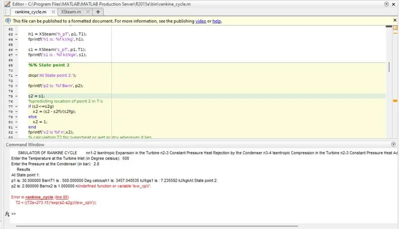
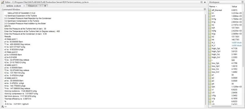
OUTPUT:-

PLOTS:-