Project 2 - Rankine cycle Simulator
RANKINE CYCLE SIMULATOR
OBJECTIVE:
To write a MATLAB code to create a Rankine cycle simulator based on the inputs provided by the user for the turbine inlet temperature, pressure and condenser outlet pressure.
RANKINE CYCLE:
The Rankine cycle is a cycle that converts heat into work. The heat is supplied externally to a closed loop, which usually uses water. This cycle generates most of the electric power used throughout the world.
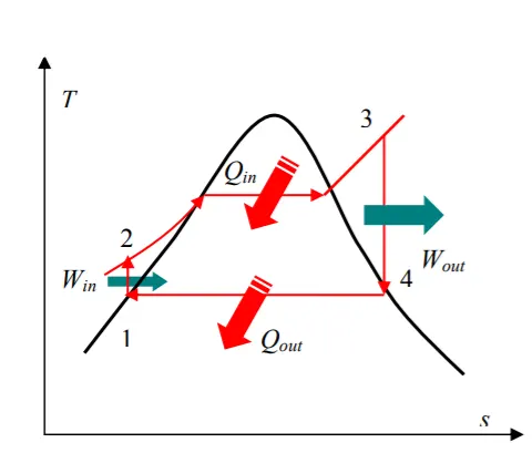
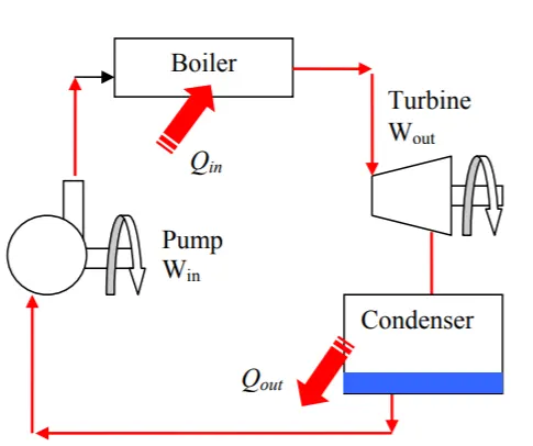
In an ideal Rankine cycle, we have the four reversible processes listed below
- Isentropic compression (1-> 2): Water enters the pump (1) as the saturated liquid and is compressed isentropically by the pump to reach the operating pressure of the boiler (2).
- Constant Pressure heat addition (2-> 3): Compressed water from the pump (2) enters the boiler & leaves the boiler as superheated vapour (3).
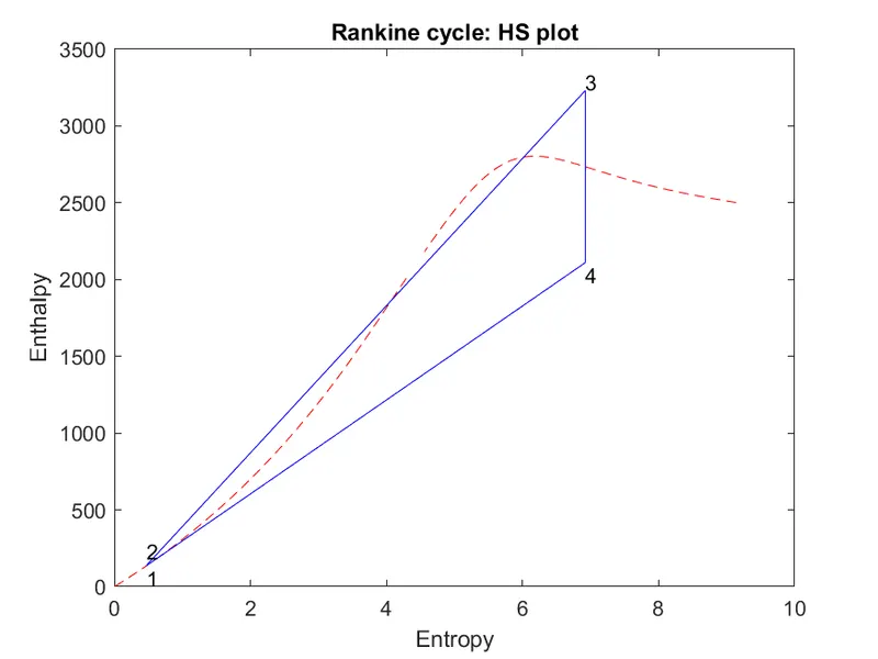
- Isentropic expansion (3 -> 4): Superheated vapour (3) expands in the turbine isentropically which produces work to the wet vapour (4) with certain percentage of water & vapour.
- Constant Pressure heat rejection (4 -> 1): Wet vapour (4) enters the condenser & leaves the condenser as saturated vapour (1) to enter the pump.
SOLUTION PROCEDURE
- User inputs has been received for the turbine inlet temperature, pressure and condenser outlet pressure.
- Entropy & Enthalpy of the superheated steam is obtained from the Xsteam function for the inlet of the turbine.
- Enthalpy of the superheated steam is obtained by the fraction of the vapour & gas from the entropy value at the state variable 2.
- Entropy, Temperature, volume & Enthalpy of the Saturated water is obtained from the Xsteam function for the inlet of the pump.
- Entropy & Temperature of the pressured water is obtained from the Xsteam function for the inlet of the boiler.
- Net work done by the rankine cycle is work done used by the pump subtracted from the work done produced by the turbine.
- Heat input in the boiler & Heat output in the condenser is estimated.
- Efficiency & SSC is calculated by the above parameters.
- Plots of TS & HS for rankine cycle & Results are printed in the command window.
CODE REFERENCE:
clear all
close all
clc

%Inputs
%turbine inlet temp: 400 deg C
%turbine inlet pressure: 30 bars
%turbine outlet pressure = Condenser inlet pressure = 0.05 bars
disp('RANKINE CYCLE')
fprintf('1-2: Isentropic pump, work input : Pump\n2-3: Constant pressure heat addition : Boiler\n3-4: Isentropic turbine, work output : Turbine\n4-1: Constant pressure hear rejection : Condenser\n')

promp1="Enter the turbine inlet temperature(deg C):";
x1=input(promp1,"s");
promp2="Enter the turbine inlet pressure(bars):";
x2=input(promp2,"s");
promp3="Enter the turbine outlet pressure(bars):";
x3=input(promp3,"s");
t3=str2num(x1);
p3=str2num(x2);
p4=str2num(x3);
%Since condenser work is constant pressure heat rejection
p1=p4;
%Since boiler work is constant pressure hear addition
p2=p3;

%at stage 3 : super heated steam
%known pressure & T(input), to find S,H
s3=XSteam('s_pt',p3,t3);
h3=XSteam('h_pt',p3,t3);

%at stage 4:wet vapour
%known pressure & S (since turbine works isentropically),
%to find H
s4=s3;
s4_f=XSteam('sL_p',p4);
s4_g=XSteam('sV_p',p4);
h4_f=XSteam('hL_p',p4);
h4_g=XSteam('hV_p',p4);
x4=(s4-s4_f)/(s4_g-s4_f);
h4=h4_f+(x4*(h4_g-h4_f));


%at stage 1 : saturated liquid
%known pressure, to find T,S,H
h1=XSteam('hL_p',p1);
s1=XSteam('sL_p',p1);
t1=XSteam('tsat_p',p1);
t4=t1;
v1=XSteam('vL_p',p1);

%at stage 2 : saturated liquid at high pressure
%known pressure & S(since pump works isentropically), to find T,H
s2=s1;
h2_test=XSteam('h_ps',p2,s2);
Cp4=XSteam('Cp_ps',p2,s2);
Cv4=XSteam('Cv_ps',p2,s2);
gamma=Cp4/Cv4;
t2=t1/((p1/p2)^((gamma-1)/gamma));

%Temperature details for plotting the curves
t23_v=XSteam('Tsat_p',p3);
s23_v=XSteam('sv_p',p3);
s23_l=XSteam('sL_p',p3);
t2_l=t23_v;

%Work done
W_t=h3-h4;
W_p=v1*((p2-p1)*100);
h2=h1+W_p;
W_net=W_t-W_p;
%Heat input in the boiler
Q_in=h3-h2;
%Heat output in the condenser
Q_out=h4-h1;
%Efficiency
eff=(W_net/Q_in)*100;
%SSC :KJ/Kwh
SSC=(3600/W_net);

%getting points for the water vapour curve
Temperature_array=linspace(0,600,1000);
for i=1:length(Temperature_array)
    Entropy_array_l(i)=XSteam('sL_T',Temperature_array(i));
    Entropy_array_v(i)=XSteam('sV_T',Temperature_array(i));
    Enthalpy_array_l(i)=XSteam('hL_T',Temperature_array(i));
    Enthalpy_array_v(i)=XSteam('hV_T',Temperature_array(i));
end
%plotting the water vapour curve
plot(Entropy_array_v,Temperature_array,LineStyle="--",Color=[1 0 0])
hold on;
plot(Entropy_array_l,Temperature_array,LineStyle="--",Color=[1 0 0])
%plotting the TS diagram of rankine cycle
plot([s1,s2],[t1 t2],Color=[0 0 1])
plot([s2,s23_l],[t2 t2_l],Color=[0 0 1])
plot([s23_l,s23_v],[t2_l,t23_v],Color=[0 0 1])
plot([s23_v,s3],[t23_v,t3],Color=[0 0 1])
plot([s3,s4],[t3 t4],Color=[0 0 1])
plot([s4,s1],[t4 t1],Color=[0 0 1])
%marking
text(s1,t1,'1','VerticalAlignment','top')
text(s2,t2,'2','VerticalAlignment','bottom')
text(s3,t3,'3','VerticalAlignment','baseline')
text(s4,t4,'4','VerticalAlignment','top')
xlabel('Entropy')
ylabel('Temperature')
title('Rankine cycle: TS plot')
hold off
saveas(gcf,'Rankine_cycle_TS_plot.png')

%plotting the water vapour curve
f2=figure()
plot(Entropy_array_v,Enthalpy_array_v,LineStyle="--",Color=[1 0 0])
hold on;
plot(Entropy_array_l,Enthalpy_array_l,LineStyle="--",Color=[1 0 0])
%plotting the hS diagram of rankine cycle
plot([s1,s2],[h1 h2],Color=[0 0 1])
plot([s2,s3],[h2 h3],Color=[0 0 1])
plot([s3,s4],[h3 h4],Color=[0 0 1])
plot([s4,s1],[h4 h1],Color=[0 0 1])
%marking
text(s1,h1,'1','VerticalAlignment','top')
text(s2,h2,'2','VerticalAlignment','bottom')
text(s3,h3,'3','VerticalAlignment','baseline')
text(s4,h4,'4','VerticalAlignment','top')
xlabel('Entropy')
ylabel('Enthalpy')
title('Rankine cycle: HS plot')
hold off
saveas(gcf,'Rankine_cycle_HS_plot.png')


%RESULTS PRINTING\
disp('*****************RESULTS**********************')
Description={'State point 1';'State point 2';'State point 3';'State point 4'}
Pressure=[p1;p2;p3;p4]
Temperature=[t1;t2;t3;t4]
Entropy=[s1;s2;s3;s4]
Enthalpy=[h1;h2;h3;h4]

T=table(Description,Pressure,Temperature,Entropy,Enthalpy)

%Properties
fprintf('Work done by the pump:%f KJ\n',W_p)
fprintf('Work produced by the turbine:%f KJ\n',W_t)
fprintf('Net work done by the Rankine cycle:%f KJ\n',W_net)
fprintf('Efficiency of the Rankine cycle:%5.3f %%\n',eff)
fprintf('SSC :%f kg/kWh\n',SSC)
RESULTS:
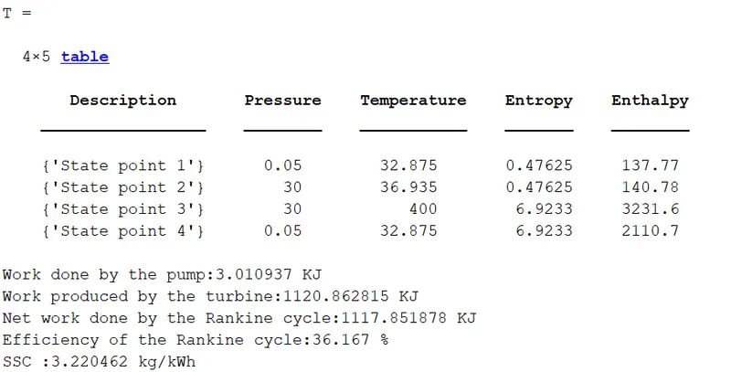
- Results displayed in the command window
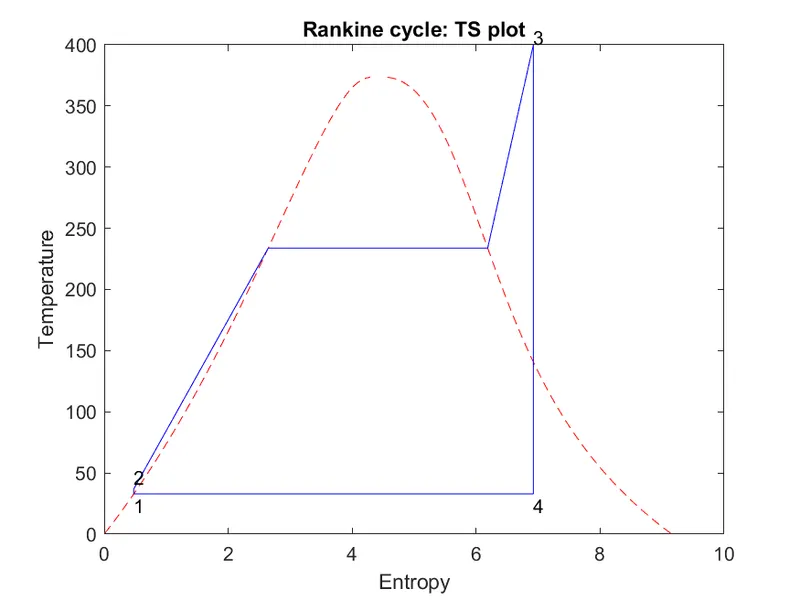
- Plots of TS plot
- Plots of HS plot
REFERENCES
https://www.engineersedge.com/thermodynamics/temp_enthalpy_th_diagram.htm
https://ch.mathworks.com/help/matlab/ref/table.html
https://en.wikipedia.org/wiki/Saturation_vapor_curve
https://www.sfu.ca/~mbahrami/ENSC%20461/Notes/Vapor%20Power%20Cycles.pdf