Project 2 - Rankine cycle Simulator

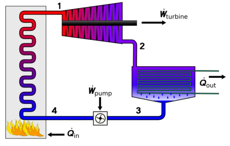
• 1-2 Isentropic Expansion. The vapor is expanded in the turbine, thus producing work that may be converted to electricity. In practice, the expansion is limited by the temperature of the cooling medium and by the erosion of the turbine blades by liquid entrainment in the vapor stream as the process moves further into the two-phase region. Exit vapor qualities should be greater than 90%.
• 2-3 Isobaric Heat Rejection. The vapor-liquid mixture leaving the turbine is condensed at low pressure, usually in a surface condenser using cooling water. In well-designed and maintained condensers, the pressure of the vapor is well below atmospheric pressure, approaching the saturation pressure of the operating fluid at the cooling water temperature.
• 3-4 Isentropic Compression. The pressure of the condensate is raised in the feed pump. Because of the low specific volume of liquids, the pump work is relatively small and often neglected in thermodynamic calculations.
• 4-1 Isobaric Heat Transfer. High-pressure liquid enters the boiler from the feed pump and is heated to saturation temperature. Further addition of energy causes evaporation of the liquid until it is fully converted to saturated steam.

FORMULAE:

`eta=W_(NET)/Q_(IN)=(W_t-W_p)/(Q_(IN))`

where,

• `Q_(IN)="Input heat"`
• `W_(NET)=W_t-W_p="Turbine work - Pump work"`

`"Back Work Ratio"=W_p/W_t`

Stepwise explanation of the code:

• Initially clear the command window.
• Take the inputs of inlet pressure, outlet pressure, and turbine inlet temperature.
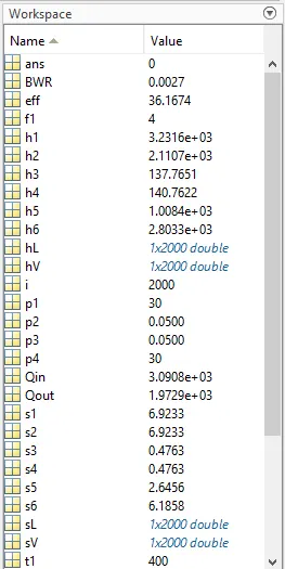
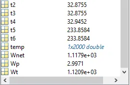
• Using XSteam() function, calculate the pressure, temperature, enthalpy, and entropy at different state points
• Using these values calculate Net work output, Back work ratio, and Efficiency of the Rankine cycle.
• To get the coordinates for the saturation curve, use an array of temperatures using the linspace() function.
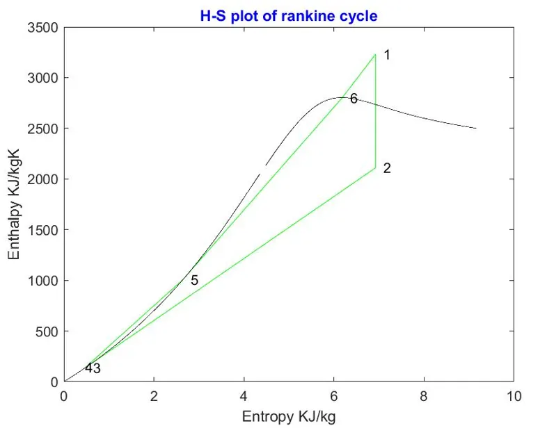
• Plot T-s and h-s plots.
• Finally, display the necessary values calculated in the command window.

PROGRAM CODE:

clear all
close all
clc

disp(' ')
fprintf('------Rankine cycle simulator------nn')
p1 = input('Enter the inlet pressure: ');
p2 = input('Enter the outlet pressure: ');
t1 = input('Enter the turbine inlet temperature: ');

%state point 1
s1 = XSteam('s_pt',p1,t1);
h1 = XSteam('h_pt',p1,t1);

%state point 2
s2 = s1;
t2 = XSteam('T_ps',p2,s2);
h2 = XSteam('h_ps',p2,s2);

%state point 3
p3 = p2;
t3 = XSteam('Tsat_p',p3);
s3 = XSteam('sL_p',p3);
h3 = XSteam('hL_p',p3);

%state point 4
p4 = p1;
s4 = s3;
t4 = XSteam('T_ps',p4,s4);
h4 = XSteam('h_ps',p4,s4);

%pressure along this path is constant
h5 = XSteam('hL_p',p1);
h6 = XSteam('hV_p',p1);
s5 = XSteam('sL_p',p1);
s6 = XSteam('sV_p',p1);
t5 = XSteam('Tsat_p',p1);
t6 = t5;

%state point display in command window
disp(' ')
fprintf('nRESULTSnn')
fprintf([' at STATE point 1: n'...
    '   P1 is : %2.2f bar n'...
    '   T1 is : %f C n'...
    '   S1 is : %f KJ/kgK n'...
    '   H1 is : %f KJ/kgK nn'],p1,t1,s1,h1)

fprintf([' at STATE point 2: n'...
    '   P2 is : %2.2f bar n'...
    '   T2 is : %f C n'...
    '   S2 is : %f KJ/kgK n'...
    '   H2 is : %f KJ/kgK nn'],p2,t2,s2,h2)

fprintf([' at STATE point 3: n'...
    '   P3 is : %2.2f bar n'...
    '   T3 is : %f C n'...
    '   S3 is : %f KJ/kgK n'...
    '   H3 is : %f KJ/kgK nn'],p3,t3,s3,h3)

fprintf([' at STATE point 4: n'...
    '   P4 is : %2.2f bar n'...
    '   T4 is : %f C n'...
    '   S4 is : %f KJ/kgK n'...
    '   H4 is : %f KJ/kgK n'],p4,t4,s4,h4)

%calculations
Qin = h1-h4;
Wt = h1-h2;
Qout = h2-h3;
Wp = h4-h3;
Wnet = Wt-Wp;

%efficiency
eff = (1-(Qout/Qin))*100;

%back work ratio
BWR = Wp/Wt;

%displaying the results
fprintf(['nNet Work output: %f KJ/kgKn'...
    'Back work ratio is %f KJ/kgn'...
    'Efficiency of the rankine cycle: %f%%n'],Wnet,BWR,eff)

%calculation of enthalpy and entropy for saturation curve
temp = linspace(0,375,2000);
for i = 1:length(temp)
    hV(i) = XSteam('hV_T',temp(i));
    hL(i) = XSteam('hL_T',temp(i));
    sV(i) = XSteam('sV_T',temp(i));
    sL(i) = XSteam('sL_T',temp(i));
end

%plotting
%T-s plot
figure(1)
plot([s1,s2],[t1,t2],[s2,s3],[t2,t3],[s3,s4],[t3,t4],[s4,s5],[t4,t5],[s5,s6],[t5,t6],[s6,s1],[t6,t1],'color','r')
%axis([-3 10 0 100])
text(s1,t1,'  1')
text(s2,t2,'  2')
text(s3,t3,'  3')
text(s4,t4,'4')
text(s5,t5,'  5')
text(s6,t6,'  6')
%to draw vapour dome
hold on
plot(sL,temp,'color','black')
plot(sV,temp,'color','black')
xlabel('Entropy KJ/kg')
ylabel('Temperature C')
title('T-S plot of rankine cycle','color','b')

%h-s plot
figure(2)
plot([s1,s2],[h1,h2],[s2,s3],[h2,h3],[s3,s4],[h3,h4],[s4,s5],[h4,h5],[s5,s6],[h5,h6],[s6,s1],[h6,h1],'color','g')
text(s1,h1,'  1')
text(s2,h2,'  2')
text(s3,h3,'  3')
text(s4,h4,'4')
text(s5,h5,'  5')
text(s6,h6,'  6')
%to draw vapour dome
hold on
plot(sL,hL,'color','black')
plot(sV,hV,'color','black')
xlabel('Entropy KJ/kg')
ylabel('Enthalpy KJ/kgK')
title('H-S plot of rankine cycle','color','b')

%openening a file to write the results
f1 = fopen('Results.txt','w');
fprintf(f1,'Net Work output: %f KJ/kgK nBack work ratio is %f KJ/kg nEfficiency of the rankine cycle: %f%%',Wnet,BWR,eff);
fclose(f1);
%dumping the plots in that folder
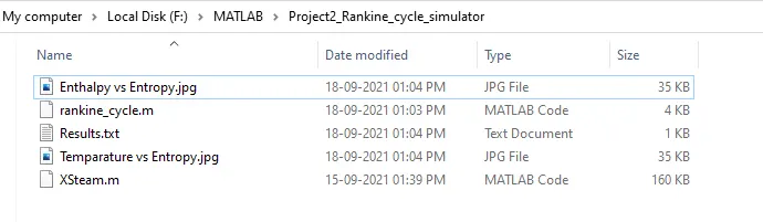
saveas(1,'Temparature vs Entropy','jpg')
saveas(2,'Enthalpy vs Entropy','jpg')

SYNTAX:

XSteam():

XSteam takes 2 or 3 arguments. The first argument must always be the steam table function you want to use. The other arguments are the inputs to that function.

First the wanted property then a _ then the wanted input properties. Example. T_ph is temperature as a function of pressure and enthalpy.

Example: XSteam('h_pt',1,20) Returns the enthalpy of water at 1 bar and 20 degC.

Example: XSteam('TSat_p',1) Returns the saturation temperature of water at 1 bar.

COMMAND WINDOW:

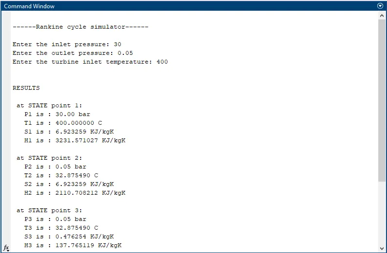
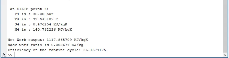
PLOTS FOR THE ABOVE CODE:

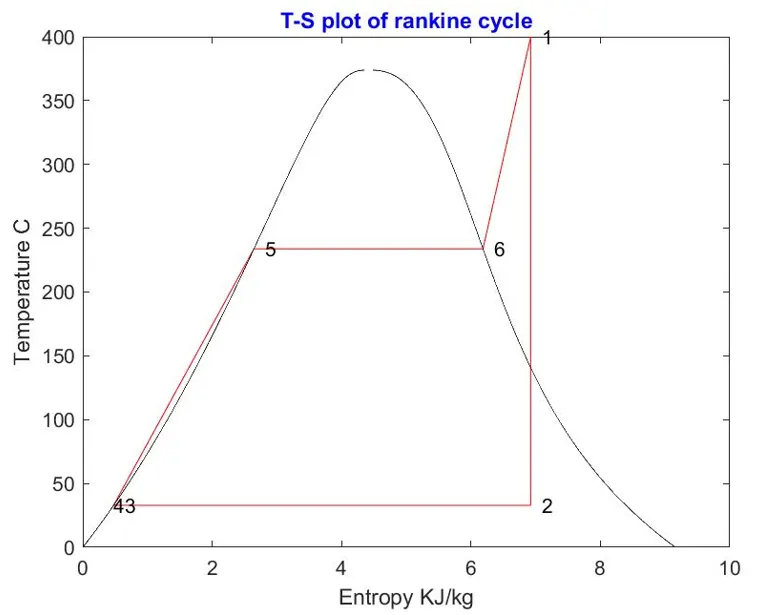
Temperature vs Entropy:

Enthalpy vs Entropy:

WORKSPACE:

FOLDER:

RESULT AND CONCLUSION:

The efficiency of the Rankine cycle is found out to be 36.167%.

By changing the input values of pressure and temperature, different plots are obtained. XSteam provides accurate steam and water properties from 0 - 1000 bar and from 0 - 2000 deg C according to the standard IAPWS IF-97.