Project 2 - Rankine cycle Simulator
AIM:
- To create a non-ideal Rankine Cycle Simulator using and studying the rankine cycle process.
- To calculate the state points of the Rankine Cycle based on user inputs.
- Plotting the corresponding T-s and h-s plots for the given set of inputs.
RANKINE CYCLE:
Rankine cycle is an idealized thermodynamic cycle of a constant pressure heat engine that converts part of heat into mechanical work. In this cycle the heat is supplied externally to a closed loop, which usually uses water (in a liquid and vapor phase) as the working fluid. In contrast to the brayton cycle, the working fluid in the rankine cycle undergo the phase change from a liquid to vapor phase and vice versa. The cycle that results to overcome impractilaties is the Rankine cycle, which is the ideal cycle for vapor
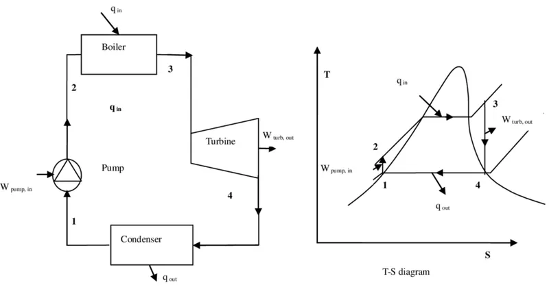
power plants. The ideal Rankine cycle does not involve any internal irreversibilities and consists of the following four processes:
1-2 Isentropic compression in a pump
2-3 Constant pressure heat addition in a boiler
3-4 Isentropic expansion in a turbine
4-1 Constant pressure heat rejection in a condenser
Isentropic Compression (1 to 2):
In this stage, a pump uses to transfer the water or other working medium from the water body (canal or tank etc.) into the boiler. The pump requires a small amount of energy for initial pumping. It pumps the fluid by increasing the pressure of the fluid, but fluid entropy remains the same. For initial pumping, the work done on the pump is given below:
Constant Pressure Heat Addition Process (2 to 3):
As the water is delivered into the boiler, an external heat source provides heat to the boiler. The boiler heated the water at constant pressure and converts it into dry saturated vapour (steam). During this process, the enthalpy of the liquid changes, and pressure remains constant.
Isentropic Expansion (3 to 4):
After the constant pressure heat addition process, the steam enters into the turbine area, where it expands. As the steam expands, it strikes with the turbine blades, which convert the thermal energy of the steam into rotational energy (mechanical work). As the turbine blades are rotated, they also rotate a crankshaft that further rotates the coil of the generator. As the coil rotates in a magnetic field, it produces electricity. During this whole process, the pressure and temperature of the steam decrease; due to that, some condensation can happen.
Constant Pressure Heat Rejection Process (4 to 1):
The vapour or steam enters the condensate tank after the expansion process. In this condensation process, the vapour is condensed to convert it into saturated liquid. During this process, the vapour rejects heat, but its liquid pressure remains the same.
One of the major advantages of the rankine cycle is that the compression process in the pump takes place on a liquid. By condensing the working steam to a liquid (inside a condenser) the pressure at the turbine outlet is lowered and the energy required by the feed pump consumes only 1% to 3% of the turbine output power and these factors contribute to a higher efficiency for the cycle, the rankine cycle is the fundamental operating cycle of all thermal power plants.
CODE WRITTEN IN MATLAB:
clear all
close all
clc

%displaying the cycle name and stages

fprintf('                     RANKINE CYCLE SIMULATOR                 ')

fprintf('\n')

disp('1-2 Isentropic compression by pump')
disp('2-3 Heat addition at const.pressure by boiler')
disp('3-4 Isentropic expansion by turbine')
disp('4-1 Heat rejection at const.pressureby condenser')

%User giving inputs
fprintf('\n')

T3 = input('Enter the turbine inlet temperature(deg C):'); %temperature entering turbine

p3 = input('Enter the turbine inlet pressure(bar):');    %pressure at turbine

p4 = input('Enter the condenser inlet pressure(bar):');  %pressure at condenser


%saturated temperature for turbine inlet pressure

T2 = XSteam('Tsat_p',p3);


%state point at 1

p1 = p4 ; %since heat rejection at constant pressure

h1 = XSteam('hL_p',p1); %enthalpy at p1,liquid phase

h_g = XSteam('hV_p',p1);%enthalpy at p1,gaseous phase

v1 = XSteam('vL_p',p1);%specific volume at p1

T1 = XSteam('Tsat_p',p1);%temperature of liquid  entering pump


sf1 = XSteam('sL_p',p1);%entropy for pressure 1

s1 = sf1;


%state property at point 2

p2 = p3 ; %simce heat addition at constant pressure

W_pump = v1*(p2-p1)*100; %work done on pump,w = pv

h2 = h1 + W_pump;

s2 = s1;

sf2 = XSteam('sL_p',p2);

cp2 = XSteam('CpL_p',p2); %specific heat at point2 for the pressure

tsat = XSteam('Tsat_p',p2);

t2 = (tsat+273.15)/(exp((sf2-s2)/cp2));

T2 = t2 - 273.15; %calculation of  temperature at point2


%state property at point 3

h3 = XSteam('h_pT',p3,T3);

s3 = XSteam('s_pT',p3,T3);  %calculating entropy


%state property at 4

s4 = s3  ;  %isentropic expansion


sf4 = XSteam('sL_p',p4);

sg4 = XSteam('sV_p',p4);

sfg4 = sg4-sf4;


x = (s4 - sf4)/sfg4;   %calculating dryness fraction

h4 = h1 + x*(h_g - h1);


if(s4<=sg4) %path followed for expansion may differ to get that we use for loop

x4 = x;

else
    x4 = 1;

end

ts4 = XSteam('Tsat_p',p4);

if(x4<1)

    T4 = ts4; %value of temperature differ with respect to dryness fraction

else
cp4 = XSteam('CpV_p',p4);

t4 = (exp((s4-sg4)/cp4))*(ts4+273.15);

T4 = t4 - 273.15;

end


%effeciency calculation

q_out = h4-h1;

q_in = h3 - h2;

W_turbine = h3 - h4;


%calculation of thermal effeciency

thermal_eff = (1 - (q_out/q_in))*100;

%net work from the cycle

W_net = W_turbine - W_pump;

%another formulae to calculate effeciency

thermeff = W_net/q_in;

 %calculating back work ration

Rbw = W_pump/W_turbine;

%plotting T-S

title('T-S diagram')

xlabel('Entropy KJ/Kg')

ylabel('Temperature deg.celsius')

%points to draw saturated liquid and vapour curve

T2_3 = XSteam('Tsat_p',p3);

T3_3 = T2_3;

s2_3 = XSteam('sL_p',p2);

hf2 = XSteam('hL_p',p2);

h2_3 = hf2;

s3_3 = XSteam('sV_p',p3);

h3_3 = XSteam('hV_p',p3);

T4_3 = XSteam('T_ps',p4,s4);

p = 0.01:400;

for i = 1:length(p)

    T(i) = XSteam('Tsat_p',p(i));
    sf(i) = XSteam('sL_p',p(i));
    sg(i) = XSteam('sV_p',p(i));
    hf(i) = XSteam('hL_p',p(i));
    hg(i) = XSteam('hV_p',p(i));

end

figure(1)

hold on

%plotting the dome shaped saturated curves

plot(sf,T,'c','linewidth',1)
plot(sg,T,'c','linewidth',1)

%[1-2] isentropic compression

plot([s1 s2],[T1 T2],'y','linewidth',2)

text(s1,T1,'1','fontsize',10)

text(s2,T2,'2','fontsize',10)

Tr = linspace(T2,T3_3,20);
hr = linspace(h2,hf2,20);
for j = 1:length(hr)

    sr(j) = XSteam('s_ph',p2,hr(j));

end
plot(sr,Tr,'k','linewidth',2)

sp1 = linspace(s2,s2_3,500);

for k = 1:length(sp1)

    Tp1(k) = XSteam('T_ps',p3,sp1(k));

end

plot(sp1,Tp1)

%[2-3] constant heat addition

plot([s2_3 s3_3],[T2_3,T3_3],'r','linewidth',2)

text(s2_3,T2_3,"2'",'fontsize',10)

%creating array of points from saturated vapour and superheated vapour

sb1 = linspace(s3_3,s3,100);

Te1 = linspace(T3_3,T3,100);

plot(sb1,Te1,'r','linewidth',2)

text(s3_3,T3_3,"3'",'fontsize',10)

%[3-4] isentropic expansion

plot([s3 s4],[T3 T4],'b','linewidth',2)

text(s3,T3,'3','fontsize',10)

% [4-1] constant pr heat rejection

if(x4<1)

    str2 = 0;

    plot(s4,T4,'.')

    plot([s4 s1],[T4,T1],'r','linewidth',2)

else
    str2 = linspace(s4,sg4,500);

    for m = 1:length(str2)

        Tt2 = XSteam('T_ps',p4,str2(m));

    end

    plot(str2,Tt2)

    plot([sg4 s1],[T1 T1],'r','linewidth',2)
end
   text(s4,T4,'4','fontsize',10)

  %plotting h-s:

  figure(2)

  hold on

  title('H-S diagram')

  xlabel('Entropy KJ/Kg')

  ylabel('Enthalpy KJ/Kg ')

  plot(sf,hf,'b','linewidth',1)

  plot(sg,hg,'b','linewidth',1)

  plot([s1 s2 s3 s4 s1],[h1 h2 h3 h4 h1],'r','linewidth',2)

  %naming the points

  text(s1,h1,'1','fontsize',10)

  text(s2,h2+90,'2','fontsize',10)

  text(s3,h3,'3','fontsize',10)

  text(s4,h4,'4','fontsize',10)


  %%display state points in command window


  fprintf('   Results    \n ')

  fprintf('\n')

  fprintf('At point 1,the state property \n')
  fprintf('p1 = %0.3f bar \n',p1)
  fprintf('T1 = %0.3f oC \n',T1)
  fprintf('H1 = %0.3f KJ/Kg \n',h1)
  fprintf('S1 = %0.3f KJ/Kgk \n',s1)

  fprintf('\n')

   fprintf('At point 2,the state property \n')
  fprintf('p2 = %0.3f bar \n',p2)
  fprintf('T2 = %0.3f oC \n',T2)
  fprintf('H2 = %0.3f KJ/Kg \n',h2)
  fprintf('S2 = %0.3f KJ/Kgk \n',s2)

  fprintf('\n')

   fprintf('At point 3,the state property \n')
  fprintf('p3 = %0.3f bar \n',p3)
  fprintf('T3 = %0.3f oC \n',T3)
  fprintf('H3 = %0.3f KJ/Kg \n',h3)
  fprintf('S3 = %0.3f KJ/Kgk \n',s3)

  fprintf('\n')

   fprintf('At point 4,the state property \n')
  fprintf('p4 = %0.3f bar \n',p4)
  fprintf('T4 = %0.3f oC \n',T4)
  fprintf('H4 = %0.3f KJ/Kg \n',h4)
  fprintf('S4 = %0.3f KJ/Kgk \n',s4)

   fprintf('\n')

   fprintf('The thermal effeciency is : %0.3f % \n',thermal_eff)

  fprintf('\n')

  fprintf('The back work ratio is : %f \n',Rbw)

  fprintf('The net work output: %f KJ \n',W_net)
EXPLANATION OF THE CODE:
step1: Clearing the previous command and outputs . Display the name of cycle and the process in the cycles by disp command.Using fprintf get the inputs from the user when the code is executed.
step2: We had the inputs of turbine inlet pressure ,temperature and condenser pressure from the user .By using that we have to calculate the state points of every stage.
step3:At point 1 the cuve will be in liquid phase which will be the inlet fluid for pump ,since the heat rejection takes place at constant pressure the pressure at point 1 will be equal to condenser pressure. To get the values we use a file XSteam which is more or less similar to steam table.The syntax to get the value is coded above.
step4:We have to get four properties for each point ,pressure,temperature,enthalpy and entropy.At point 2 the working fluid enters the boiler for heat addition after compression from pump the pressure got increased which will be constant throughout heat addition.After heat addition fluid enters for expansion where the shaft rotates from that we get electrical output.
step5:While changing phase the fluid follows change in entropy with constant temperature i.e the line will be horizontal inside the dome curve.We have to find the saturation temperature,where the points which lie on the saturation liquid and vapor lines use L for liquid and V for vapour.
step6:By successfully completing the calculation,we start to calculate the thermal effeciency, net work,back work ratio using the respective formula which is learned in thermodynamics
using the values we calculated
step7:The path following the expansion curve may differ with respect to inputs ,it may be of saturated vapour or superheated vapor so we need to calculate dryness fraction x for that point,the dryness fraction is nothing but the measure of moisture content,it ranges from 0 to 1.
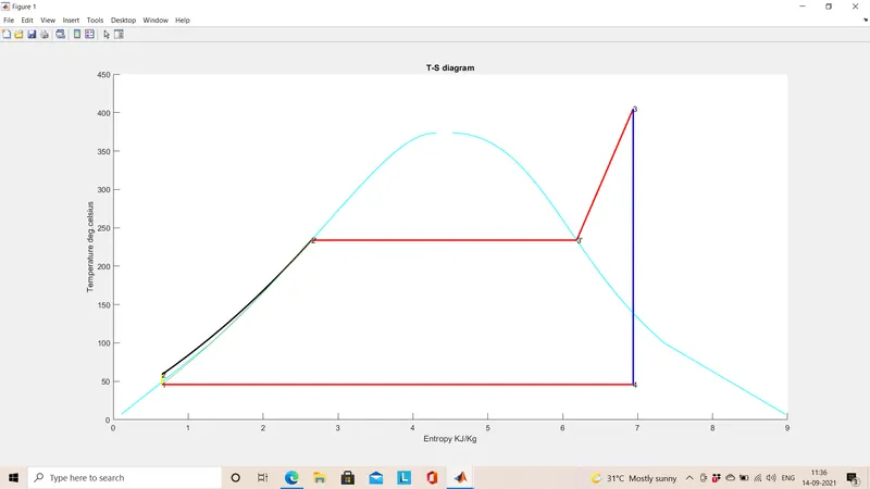
step8: Then we write the code for ploting temperature and entropy using the calculated values,first we calculate the saturated vapor and liquid lines using entropy liquid phase and vapor phase.The cycle curve can be drawn using the values got from steam tables and some formulae.The image for t-s is attached below.
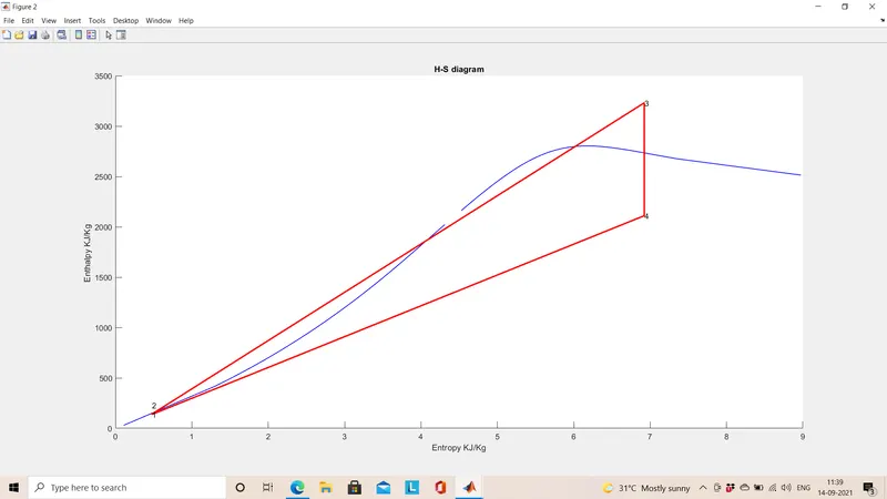
step9:Then plot the h-s diagram,the curve is for enthalpy and entropy.Label the points in the cycle using text command,the saturation line is drawn for this curve also instead of t we mention here h.
step10:Finally display the results that we calculated in the code for all the four states . Here we use \n to write the result in new line which makes the results in command window more clear and readable.
COMMANDS USED :text-It is used to write the numbers in the plot
disp-It is used to display the content we write in code in command window.
RESULTS:
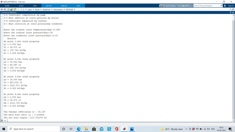
Command window showing the outputs of rankine cycle for the given inputs.
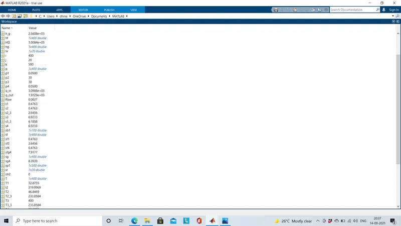
workspace:
PLOT IMAGES:
T-S:
H-S:
CONCLUSION:
The code for rankine cycle simulator is written down and executed successfully.
For the given input the T-S and H-S plot is drawn . The thermal effeciency,back work ratio and net work output is calculated.
The state points,properties of the respective points are displayed in command window successfully.
REFERENCES:
Thermal-fluid science book by yunus sengel
What is Rankine Cycle - Steam Turbine Cycle - Definition (thermal-engineering.org)
Rankine Cycle | How to Calculate the Efficiency of the Rankine Cycle? (mechanicalboost.com)
Rankine Cycle - Ideal Rankine Cycle efficiency - Mechanicaltutorial