Project 2 - Rankine cycle Simulator
"Project 2 - Rankine cycle Simulator"
Aim: To create a program for Rankine Cycle Simulator and plot T-S, H-S diagram.
Objective:
- To create a Rankine Cycle Simulator.
- To write a program for calculating the state points of the Rankine Cycle based on user inputs.
- Plot the corresponding T-S and H-S diagram for the given sets of inputs.
Basic Theory:
The Rankine cycle is an idealized thermodynamic cycle describing the process by which certain heat engines, such as steam turbines or reciprocating steam engines, allow mechanical work to be extracted from a fluid as it moves between a heat source and heat sink.
In Rankine Cycle the heat energy is supplied to the system via a boiler where the working fluid (typically water) is converted to a high-pressure gaseous state (steam) in order to turn a turbine. After passing over the turbine the fluid is allowed to condense back into a liquid state as waste heat energy is rejected before being returned to the boiler, completing the cycle. Friction losses throughout the system are often neglected for the purpose of simplifying calculations as such losses are usually much less significant than thermodynamic losses, especially in larger systems.
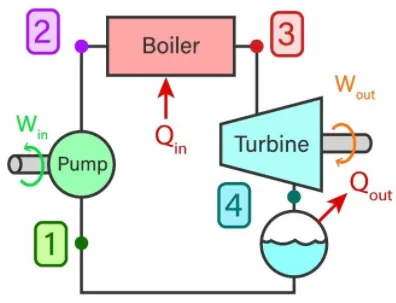
Where,
Win = Work done by pump to increase the pressure of working fluid
Wout = Output work given by turbine through rotating shaft where the dry saturated vapor expands.
Qin = Heat produced by boiler high-pressure fluid at constant pressure.
Qout = Heat given out by condenser to condense wet vapour to saturated liquid at constant pressure.
There are four main components,
- Pump (P)
- Boiler (B)
- Turbine (T)
- Condenser (C)
Pump:
- Point 1-2 indicates pump in Rankine cycle
- Work done incurs to the system.
- Pressure is increased in this stage.
Boiler:
- Point 2-3 represents the boiler in the cycle.
- Heat is added to the high pressured fluid by the boiler.
- Temperature is increased up to a boiling point.
- Water changed into vapor as its phase is changed.
Turbine:
- Point 3-4 indicates the turbine in the Rankine cycle diagram.
- Expansion of vapor happens in the turbine.
Condenser:
- Point 4-1 indicates the condenser.
- Waste heat is removed from the condenser with the help of the condensation process.
In the ideal Rankine cycle, there are four processes running, we will check each of them and what will happen in each process.
In case of the process 1 -2 – Isentropic compression
In this process, the working fluid will be pumped from low pressure to high pressure. The fluid is in the liquid form at the start of this process.
The water is heated to the saturation temperature, keeping the entropy constant.
Process 2-3 – Constant Pressure Heat Addition Process in Boiler
In case of this process, the high-pressure liquid will enter the boiler. The fluid will be heated at constant pressure with the help of an external heat source and it will become a dry saturated vapour.
The required energy needed for heating up can be calculated with the help of enthalpy entropy chart or steam tables.
Process 3-4 – Isentropic Expansion Process
The dry saturated vapour at the end of the process 2-3 will be expanded through the turbine in this process. It will generate the power.
Due to expansion the temperature and the pressure of the vapor will be decreased. Same as the above the output can be easily calculated.
Process 4-1 – Constant Pressure Heat Rejection in Condenser
In this process, the low temperature and low-pressure vapour will be condensed in the condenser. It will be converted into saturated liquid.
Equations Used:
P1 = Condenser Pressure
P2 = Pump Pressure
P3 = Boiler Pressure
P4 = Turbine Pressure
P1 = P4, from process 4-1 we can see that the pressure is constant and only heat is rejected at the condenser.
P2 = P3, from process 2-3 we can see that the pressure is constant and heat is added to the boiler.
S1 = S2, from process 1-2 we can see that the process is isentropic compression.
S3 = S4, from process 3-4 we can see that the process is isentropic expansion.
h1,h2,h3,h4 = The specific enthalpies at the state points.
s1,s2,s3,s4 = Entropies at the state points.
W = Mechanical power consumed by or provided to the system.
(i) For Boiler:-
h4 + Q1 = h1
Q1 = h1-h4
(ii) For Turbine:-
h1 = Wt + h2 (Where, Wt = Work done by the Turbine)
Wt = h1 - h2
(iii) For Condenser:-
h2 = Q2 + h3
Q2 = h2 - h3
(iv) For the feed pump:-
h3 + Wp = h4 (Where, Wp = Work done by Pump)
Wp = h4 - h3
Rankine Cycle Efficiency:-

Net Workdone = Work Extracted - Work input = Wt - Wp. Since, we provide the work input to the pump, we must remove the same amount of work from the work output we extract from the system.
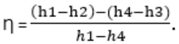
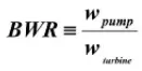
Back Work Ratio:-
Back Work Ratio is the amount of work consumed by the pump which is generated by the turbine. Lower the value of the back work ratio higher the performance of the cycle.
Given:-
In order to find state points and properties, a steam table function 'XSteam.m' was given for the use. The XSteam.m file is in following link-
https://drive.google.com/drive/folders/19CV3ld7TVy41EachgB35WlNY6yVehVqY
Given Required inputs:-
Turbine Inlet temperature = 400° C
Turbine Inlet Pressure = 30 bars
Turbine Outlet Pressure = 0.05 bars = Condenser Inlet Pressure
Matlab Program:
% A Program to simulate the Rankine Cycle Simulator

clear all
close all
clc

% Rankine Cycle Processes
fprintf('RANKINE CYCLE SIMULATOR \n')
fprintf('1-2 is Isentropic Expansion in Turbine\n')
fprintf('2-3 is Constant Pressure Heat Rejection in Condenser\n')
fprintf('3-4 is Isentropic Compression in Pump\n')
fprintf('4-1 is Constant Pressure Heat Addition in Boiler\n')

% Inputs
p1 = input('\n Presssure at the Turbine inlet (in bar) : ');
t1 = input('\n Temperature at the Turbine inlet (in degree celsius) : ');
p2 = input('\n Pressure at the Condenser inlet (in bar) :');

% At State Point 1 (Turbine Inlet)
% p1 & t1 are given
h1 = XSteam('h_pT', p1,t1);  % Enthalpy at State Point 1
s1 = XSteam('S_pT', p1,t1);  % Specific Entropy at State Point 1

% At State Point 2 (Condenser Inlet)
% p2 is given
s2 = s1;
sf2 = XSteam('sL_p',p2);     % Entropy at saturation liquid at pt. 2
sg2 = XSteam('sV_p',p2);     % Entropy at saturation vapour at pt.2
hf2 = XSteam('hL_p',p2);     % Enthalpy of saturation liquid at pt.2
hg2 = XSteam('hV_p',p2);     % Enthalpy of saturation vapour at pt.2

hfg = hg2 - hf2;
sfg = sg2 - sf2;

if s2 > sg2
    x2 = 1;    % x2 is the dryness fraction
    h2 = x2*hg2; % Enthalpy at State Point 2
else
    x2 = (s2-sf2)/(sg2-sf2);
    h2 = hf2 + (x2*(hg2-hf2));
end

% At State Point 3 (Pump Inlet)
p3 = p2;
h3 = XSteam('hl_p',p3);
s3 = XSteam('sL_p',p3);
t3 = XSteam('Tsat_p',p3);
t2 = t3;

% At State Point 4 (Boiler Inlet)
p4 = p1;
s4 = s3;
h4 = XSteam('h_ps',p4,s4);

Cp4 = XSteam('Cp_ps',p4,s4);
Cv4 = XSteam('Cv_ps',p4,s4);
lambda = Cp4/Cv4;
t4 = t3/((p3/p4)^((lambda-1)/lambda));

t5 = XSteam('Tsat_p',p1);
t6 = t5;
s5 = XSteam('sL_p',p1);
s6 = XSteam('sV_p',p1);
h5 = XSteam('hL_p',p1);
h6 = XSteam('hV_p',p1);

% Work done by the Turbine
wt = h1 - h2;

% Work done by the Pump
wp = h4 - h3;

% Net Work out put (in KJ/kg)
w = wt- wp;

% Heat in & out of the system
Q_in = h1 - h4;
Q_out = h2 - h3;

% Thermal Efficiency
Efficiency = (w/Q_in)*100;

% Steam Rate (in kg/kwh)
ssc = 3600/w;

% Back Work Ratio
BWR = (h1 - h4)/(h2 - h3);

% Plot Saturation Curve;
T = linspace(1,400,500);
for i = 1:length(T)
    hL(i) = XSteam('hL_T',T(i));
    hV(i) = XSteam('hV_T',T(i));
    sL(i) = XSteam('sL_T',T(i));
    sV(i) = XSteam('sV_T',T(i));
end

% Plotting T-S Diagram
figure(1)
hold on
title('T-S Diagram of Rankine Cycle')
plot([s1 s2],[t1 t2],'linewidth',3,'color','b')
plot([s2 s3],[t2 t3],'linewidth',3,'color','b')
plot([s3 s4],[t3 t4],'linewidth',3,'color','b')
plot([s4 s5],[t4 t5],'linewidth',3,'color','b')
plot([s5 s6],[t5 t6],'linewidth',3,'color','b')
xlabel('Entropy (in KJ/kgk)')
ylabel('Temperature (in Degree C)')
S1 = linspace(s6,s1,500);
for j = 1:length(S1)
    T1(j) = XSteam('T_ps',p1,S1(j));
end
plot(S1,T1,'linewidth',3,'color','b')
plot(sL,T,'linewidth',1.5,'color','r')
plot(sV,T,'linewidth',1.5,'color','r')

% Annotations
text(s1,t1,'1','FontSize',15)
text(s2,t2,'2','FontSize',15)
text(s3,t3,'3','FontSize',15,'verticalalignment','top')
text(s4,t4,'4','FontSize',15,'verticalalignment','bottom')
text(s5,t5,'5','FontSize',15,'verticalalignment','bottom')
text(s6,t6,'6','FontSize',15,'verticalalignment','bottom')

% Plotting H-S Diagram
figure(2)
hold on
title('H-S Diagram of Rankine Cycle')
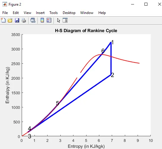
plot([s1 s2],[h1 h2],'linewidth',3,'color','b')
plot([s2 s3],[h2 h3],'linewidth',3,'color','b')
plot([s3 s4],[h3 h4],'linewidth',3,'color','b')
xlabel('Entropy (in KJ/kgk)')
ylabel('Enthalpy (in KJ/kg)')
H4 = linspace(h4,h5,500);
for k = 1:length(H4)
    S4(k) = XSteam('s_ph',p1,H4(k));
end
H6 = linspace(h6,h1,500);
for m = 1:length(H6)
    S6(m) = XSteam('s_ph',p1,H6(m));
end
plot(S4,H4,'linewidth',3,'color','b')
plot([s5 s6],[h5 h6],'linewidth',3,'color','b')
plot(S6,H6,'linewidth',3,'color','b')
plot(sL,hL,'linewidth',1.5,'color','r')
plot(sV,hV,'linewidth',1.5,'color','r')

% Annotations
text(s1,h1,'1','FontSize',15)
text(s2,h2,'2','FontSize',15)
text(s3,h3,'3','FontSize',15,'verticalalignment','top')
text(s4,h4,'4','FontSize',15,'verticalalignment','bottom')
text(s5,h5,'5','FontSize',15,'verticalalignment','bottom')
text(s6,h6,'6','FontSize',15,'verticalalignment','bottom')

% Result Window
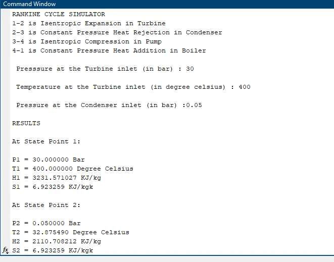
fprintf('\nRESULTS\n')
fprintf('\nAt State Point 1: \n')
fprintf('\nP1 = %f Bar\n',p1)
fprintf('T1 = %f Degree Celsius\n',t1)
fprintf('H1 = %f KJ/kg\n',h1)
fprintf('S1 = %f KJ/kgk\n',s1)

fprintf('\nAt State Point 2: \n')
fprintf('\nP2 = %f Bar\n',p2)
fprintf('T2 = %f Degree Celsius\n',t2)
fprintf('H2 = %f KJ/kg\n',h2)
fprintf('S2 = %f KJ/kgk\n',s2)

fprintf('\nAt State Point 3: \n')
fprintf('\nP3 = %f Bar\n',p3)
fprintf('T3 = %f Degree Celsius\n',t3)
fprintf('H3 = %f KJ/kg\n',h3)
fprintf('S3 = %f KJ/kgk\n',s3)

fprintf('\nAt State Point 4: \n')
fprintf('\nP4 = %f Bar\n',p4)
fprintf('T4 = %f Degree Celsius\n',t4)
fprintf('H4 = %f KJ/kg\n',h4)
fprintf('S4 = %f KJ/kgk\n',s4)

fprintf('\nWork done by Turbine is :%f KJ/kg\n',wt)
fprintf('\nWork done by Pump is :%f KJ/kg\n',wp)
fprintf('\nNet Work out put of the system is :%f KJ/kg\n',w)
fprintf('\nSpecific steam consumption :%f kg/KWh\n',ssc)
fprintf('\nThe net Thermal Efficiency of the system is :%f\n',Efficiency)
fprintf('\nThe BWR of the Rankine Cycle is :%f\n',BWR)
Code Explanation:
- The known inputs are collected initially by using the input command (p1,t1 and p2).
- By using the relations between the various properties of the ideal Rankine Cycle the values are calculated for all the state points.
- In order to obtain the values from the steam table, the function XSteam is added to the current working folder of Matlab.
- Next, by using the appropriate input parameters for the XSteam function,the required values are obtained.
- Then we have made the ''if-else'' statement for the two cases of possibility for the dryness fraction(x) one state point lying in the fluid-vapour region and the second lying in the superheat region.
- Then we have given respective equations to calculate the net work output, efficiency, steam rate per second, work done by pump and work done by turbine and Back work ratio.
- To display the vapour line we have entered the input by "linspace" command and used "for-loop".
- Then by using the "plot" command we have obtained T-S and H-S Diagram.
- Next, we have used the "text" command which displays the number for the respective state point .
- At last "fprintf"command is used to display all the values of the state point variables in the command window.
Result:
1) Temperature-Entropy diagram of Rankine Cycle:-
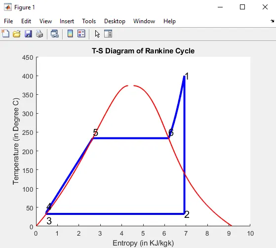
2) Enthalpy-Entropy diagram of Rankine Cycle:-
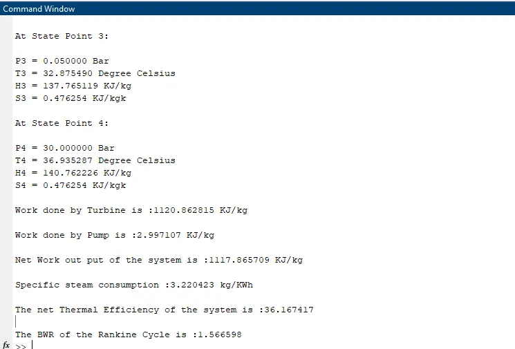
3) Command Window:-
Errors Encountered:
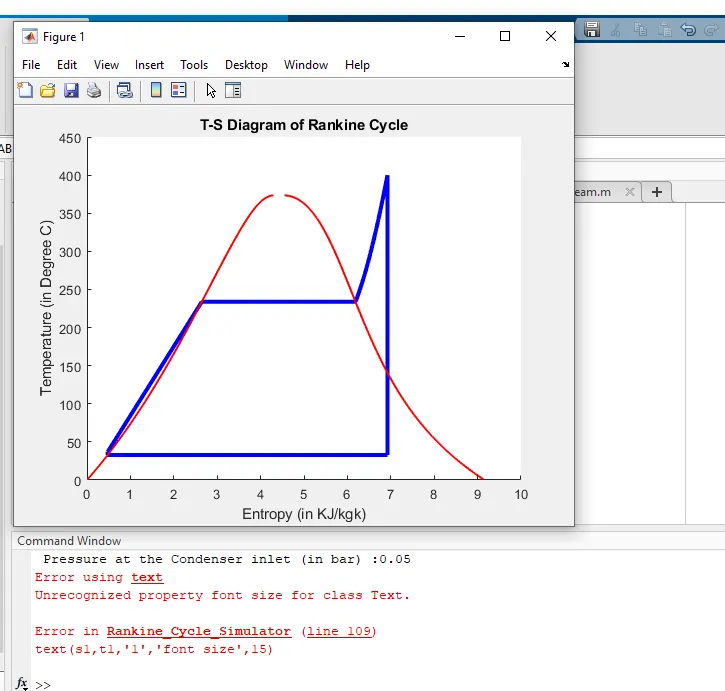
From the above plot we can clearly see that we have used wrong text command as we have used "font size" instead of "FontSize" and also for this wrong command we were not getting the H-S plot. So, for the proper execution of the code we have replaced the "font size" into "FontSize".
Conclusion:
- Thus the Net work out put and back work ratio for ideal rankine cycle was calculated by using Matlab Programming.
- Net Work out put = 1117.865709 KJ/kg
- Back Work Ratio = 1.566598
- We had plotted the diagram of T-S and H-S of Ideal Rankine Cycle.