Project 2 - Rankine cycle Simulator
AIM: To write a program of Rankine Cycle Simulator using MATLAB based on inputs.
obejctive: Plot the corresponding T-s and h-s plots for the given set of inputs.
INPUTS REQUIRED:
-
Turbine Inlet temperature = 400° C.
-
Turbine Inlet Pressure = 30 bars.
-
Turbine Outlet Pressure = 0.05 bars = Condenser Inlet Pressure.
THEORY AND EXPLANATION:
Rankine Cycle:
The Rankine cycle is a model used to predict the performance of steam turbine systems. It was also used to study the performance of reciprocating steam engines. The Rankine cycle is an idealized thermodynamic cycle of a heat engine that converts heat into mechanical work while undergoing a phase change. It is an idealized cycle in which friction losses in each of the four components are neglected. The heat is supplied externally to a closed loop, which usually uses water as the working fluid.
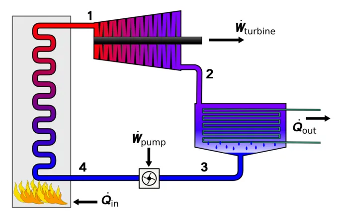
There are four processes in the Rankine cycle:
Process 1-2: Isentropic expansion in the turbine.
Process 2-3: Constant pressure heat rejection by the condenser.
Process 3-4: Isentropic compression in the pump.
Process 4-1: Constant pressure heat addition in the boiler.
Formulae:
i) For Boiler:
hf4 + Q1 = h1
Q1 = h1 - hf4
ii) For the turbine:
h1 = Wt + h2; where Wt = turbine work
Wt = h1 - h2
iii) For Condenser:
h2 = Q2 + hf3
Q2 = h2 - hf3
iv) For the feed pump:
hf3 + Wp = hf4; where Wp= pump work
Wp = hf4 - hf3
v) The thermal efficiency of the Rankine cycle:
η=Wnet/Q1
η=(Wt-Wp)/Q1
RANKINE CYCLE T-S DIAGRAM:
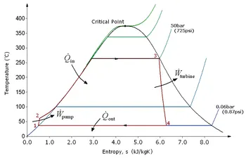
Process 1–2: Isentropic compression in pump
The working fluid is pumped from low to high pressure. As the fluid is a liquid at this stage, the pump requires little input energy.
Process 2–3: Constant pressure heat addition in boiler
The high-pressure liquid enters a boiler, where it is heated at constant pressure by an external heat source to become a dry saturated vapour. The input energy required can be easily calculated graphically, using an enthalpy–entropy chart (h–s chart, or Mollier diagram), or numerically, using steam tables.
Process 3–4: Isentropic expansion in turbine
The dry saturated vapour expands through a turbine, generating power. This decreases the temperature and pressure of the vapour, and some condensation may occur. The output in this process can be easily calculated using the chart or tables noted above.
Process 4–1: Constant pressure heat rejection in condenser
The wet vapour then enters a condenser, where it is condensed at a constant pressure to become a saturated liquid.
MATLAB CODE:
%Rankine Cycle
clear al
close all
clc
disp(' RANKINE CYCLE ');
disp('1-2 is Iscentropic Expansion in the Turbine');
disp('2-3 is Constant Pressure Heat rejection by the Condensor');
disp('3-4 is Iscentropic Expansion in the Pump');
disp('4-1 is Constant Pressure Heat addition to the Boiler');
%Inputs:
disp(' INPUTS ');
P1 = input('Enter the Pressure at turbine inlet(bar):');
T1 = input('Enter the Temperature at the Turbine inlet(degree C):');
P2 = input('Enter the Pressure at the Condensor(bar):');
%Using the XSteam functions,the enthalpy and entropy at various
%points can be calculated:
%Caluclating enthalpy(h) and entropy(s) at point 1:
h1 = XSteam('h_pT',P1,T1);
s1 = XSteam('s_pT',P1,T1);
%Caluclating pressure(P),enthalpy(h) and entropy(s) at point 2:
%Since Iscentropic Expansion:
s2=s1;
%For Iscentropic Expansion:
% wkt (T2/T1)=(P2/P1)^(1-(1/g))
g = 1.4;
power = 1-(1/g);
%Hence (T2/T1) = (P2/P1)^power:
T2 = T1*((P2/P1)^power);
h2 = XSteam('h_pT',P2,T2);
%Caluclating pressure(P),enthalpy(h) and entropy(s) at point 3:
%Since Constant Pressure Heat Removal:
P3 = P2;
T3 = T2;
h3 = XSteam('hL_T',T3);
s3 = XSteam('sL_T',T3);
%Caluclating pressure(P),enthalpy(h) and entropy(s) at point 4:
%Since Iscentropic Compression:
s4 = s3;
%Since Constant Pressure Process:
P4 = P1;
T4 = XSteam('T_ps',P4,s4);
h4 = XSteam('h_pT',P4,T4);
h41 = XSteam('hL_p',P4);
s41 = XSteam('sL_p',P4);
h42 = XSteam('hV_p',P4);
s42 = XSteam('sV_p',P4);
T41 = XSteam('T_hs',h41,s41);
T42 = XSteam('T_hs',h42,s42);
%Calculating the Entropy and Enthapy at the saturation curve:
Temp = linspace(0,500,600);
for i = 1:length(Temp)
sv(i) = XSteam('sV_T',Temp(i));
sl(i) = XSteam('sL_T',Temp(i));
hv(i) = XSteam('hV_T', Temp(i));
hl(i) = XSteam('hL_T', Temp(i));
end
%Calculating Net Work Output(W_net):
W_t = h1-h2;
W_p = h4-h3;
W_net = W_t-W_p;
%Calculating Back Work Ratio:
Bw_ratio = W_p/W_t;
%Calculating the Thermal efficiency:
Q_in = h1-h4;
eff_thermal = (W_net/Q_in)*100;
%Calculating Specific Steam Consumption:
% wkt 1J = 3600kg/s
SSC = 3600/W_net;
% Displaying Results in the command window:
disp(' Results ');
P1 = P1;
T1 = T1;
P2 = P2;
disp('At stage point 1');
n1 = sprintf('P1 is %.3f bar',P1);
disp(n1);
n2 = sprintf('T1 is %.3f C',T1);
disp(n2);
n3 = sprintf('h1 is %.3f kJ/kg',h1);
disp(n3);
n4 = sprintf('s1 is %.3f kJ/kgK',s1);
disp(n4);
disp('At stage point 2');
n11 = sprintf('P2 is %.3f bar',P2);
disp(n11);
n21 = sprintf('T2 is %.3f C',T2);
disp(n21);
n31 = sprintf('h2 is %.3f kJ/kg',h2);
disp(n31);
n41 = sprintf('s2 is %.3f kJ/kgK',s2);
disp(n41);
disp('At stage point 3');
n12 = sprintf('P3 is %.3f bar',P3);
disp(n12);
n22 = sprintf('T3 is %.3f C',T3);
disp(n22);
n32 = sprintf('h3 is %.3f kJ/kg',h3);
disp(n32);
n42 = sprintf('s3 is %.3f kJ/kgK',s3);
disp(n42);
disp('At stage point 4');
n13 = sprintf('P4 is %.3f bar',P4);
disp(n13);
n23 = sprintf('T4 is %.3f C',T4);
disp(n23);
n33 = sprintf('h4 is %.3f kJ/kg',h4);
disp(n33);
n43 = sprintf('s4 is %.3f kJ/kgK',s4);
disp(n43);
n14 = sprintf('W_t is %.3f kJ/kg',W_t);
disp(n14);
n15 = sprintf('W_p is %.3f kJ/kg',W_p);
disp(n15);
n16 = sprintf('W_net is %.3f kJ/kg',W_net);
disp(n16);
n17 = sprintf('Eff_Thermal is %.2f Percent',eff_thermal);
disp(n17);
n18 = sprintf('SSC is %.2f kg/kWh',SSC);
disp(n18);
figure(1)
plot([s1 s2],[T1 T2],[s2 s3],[T2 T3],[s3 s4],[T3 T4],[s4 s41],[T4 T41],[s41 s42],[T41 T42],[s42 s1],[T42
T1],'marker','*','color','r')
hold on
plot(sv,Temp)
plot(sl,Temp)
xlabel('Entropy-s(kJ/kgK');
ylabel('Temperature-T(K)');
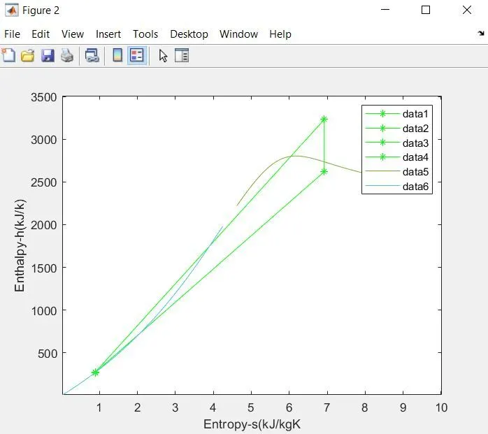
figure(2)
plot([s1 s2],[h1 h2],[s2 s3],[h2 h3],[s3 s4],[h3 h4],[s4 s1],[h4 h1],'marker','*','color','g')
hold on
plot(sv,hv)
plot(sl,hl)
xlabel('Entropy-s(kJ/kgK');
ylabel('Enthalpy-h(kJ/k)');
RESULTS AND OUTPUT:
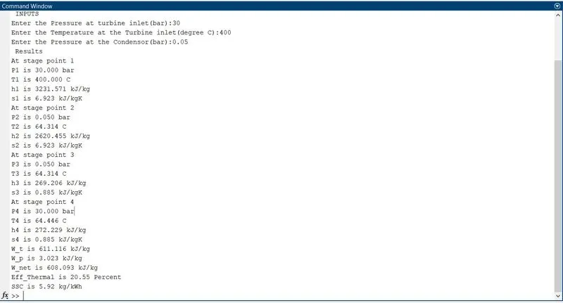
COMMAND WINDOW:
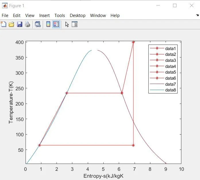
i) PLOT FOR T-S DIAGRAM:
ii) PLOT FOR H-S DIAGRAM:
Conclusion:
The performance of the Heat Engine was calculated and the following Observations were made:
- Net Work = 608.093 kJ/kg
- Thermal Efficiency = 20.55%
- Back Work Ratio = 0.4%