Project 2 - Rankine cycle Simulator

Objective :

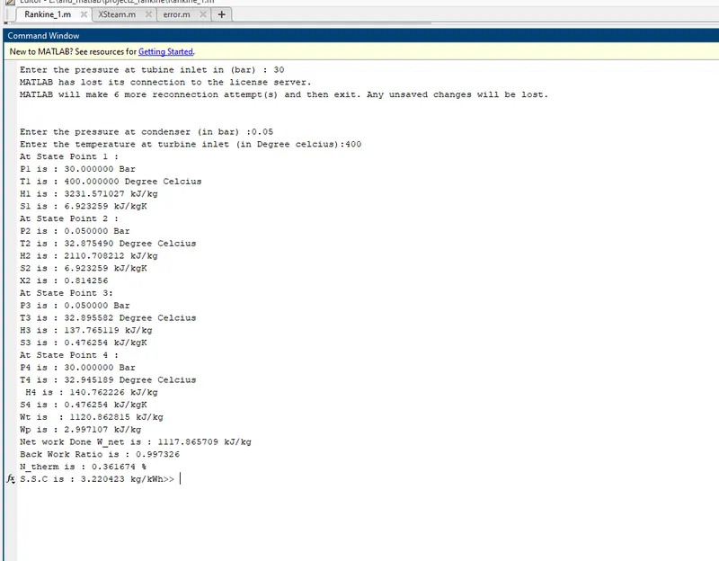
1) To write a program that calculates the state points of a Rankine Cycle based upon user input of pressure at condenser and turbine and temperature at turbine .

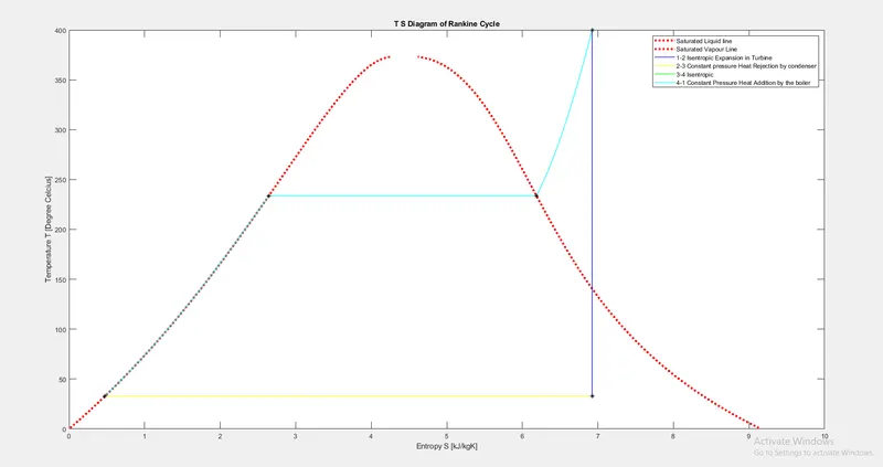
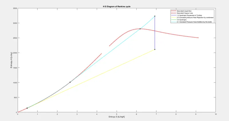
2) Plot T-S and H-S diagram for the corresponding values obtained .

Theory :

Rankine cycle is a thermodynamic cycle that is used to convert heat produced by burning a fuel into mechanical energy .

The Rankine cycle makes use of increase inpressure of a condensed fluid which is forced to vapourise in a contained vessel . The cycle begins when a fluid such as water is compressed under high pressure . This high pressure liquid is converted to vapour and this vapour is used to rotate a turbine which produces mechanical work . When the vapour is cooled, it turns into a liquid state and this cycle repeats .

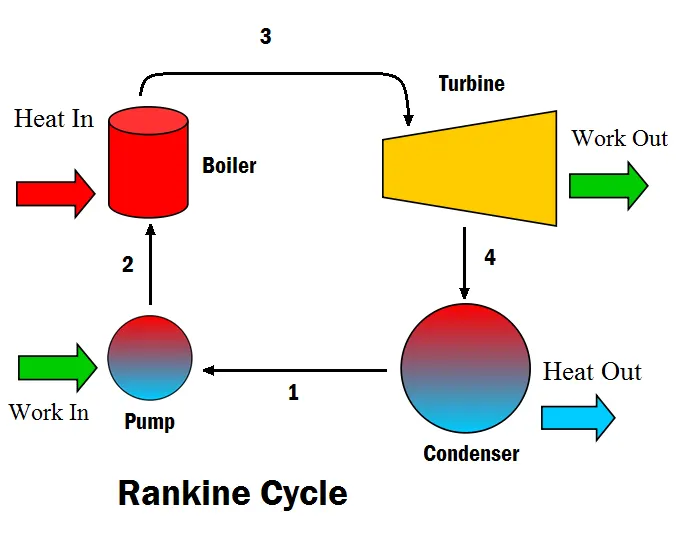
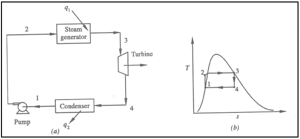
The Rankine cycle makes use of 4 main components .

a) Pump : Used to compress liquid to high pressure and feed to the boiler .

b) Boiler : The boiler converts liquid/water to vapour state .

c)Turbine : The high pressure vapour in used to rotate turbine and convert heat to mechanical or electrical energy (by connecting the turbine to a generator).

d) Condenser : The condenser is used to cool the vapour and convert it to liquid state .

Programme Logic:

clear all
close all
clc

p1=input('Enter the pressure at tubine inlet in (bar) : '); : To input turbine inlet pressure P1
p2=input('Enter the pressure at condenser (in bar) :'); : To input condenser pressure P2
t1=input('Enter the temperature at turbine inlet (in Degree celcius):'); : To input temperature at turbine inlet T1

s1=XSteam('s_pT',p1,t1); : To obtain s1 from steam table

h1=XSteam('h_pT',p1,t1); : To obtain h1 froms team table
disp('At State Point 1 : ') : To display 'At State Point 1'
fprintf('P1 is : %f Bar \n',p1 ) : To print value of p1 with SI unit
fprintf('T1 is : %f Degree Celcius \n',t1 ) : To print value of t1 with SI unit
fprintf('H1 is : %f kJ/kg \n',h1 ) : To print value of h1 with SI unit
fprintf('S1 is : %f kJ/kgK \n',s1 ) :To print value of s1 with SI unit

s2=s1; : Defining s2 as s1 since 1-2 is an isentropic process .
t2=XSteam('T_ps',p2,s2); : To obtain value of t2 based on p2 and s2 from steam table
sf=XSteam('sL_p',p2); :To obtain value of sf based on p2 from steam table
sg=XSteam('sV_t',t2); :To obtain value of sg based on t2 from steam table
sfg=sg-sf; : defining sfg as deifference between sg and sf
x=(s2-sf)/sfg; : calculating x from given formula
hf2=XSteam('hL_T',t2); : To obtain hf2 based on t2 from steam table
hg2=XSteam('hV_T',t2); : To obtain hg2 based on t2 from steam table
hfg2=hg2-hf2; : Defining hfg2 as difference between hg2 and hf2
h2=hf2+x*hfg2; : Calculating h2 from given equation
disp('At State Point 2 : ') : To display 'At State Point 2'
fprintf('P2 is : %f Bar \n',p2 ) :To print value of p2 with SI unit
fprintf('T2 is : %f Degree Celcius \n',t2 ) : To print value of t2 with SI unit
fprintf('H2 is : %f kJ/kg \n',h2 ) :To print value of h2 with SI unit
fprintf('S2 is : %f kJ/kgK \n',s2 ) :To print value of s2 with SI unit
fprintf('X2 is : %f \n',x) : To print value of x2

p3=p2; : Defining p3 as p2 since 2-3 is at constant pressure
h3=hf2; : Defining h3 as hf since it is at saturation point
t3=XSteam('T_ph',p3,h3); : To obtain t3 based on p3 and h3 from steam table
s3=XSteam('sL_p',p3); : to obtain s3 based on p3 from steam table
disp('At State Point 3: ') :To display 'At State Point 3'
fprintf('P3 is : %f Bar \n',p3 ) :To print value of p3 with SI unit
fprintf('T3 is : %f Degree Celcius \n',t3 ) :To print value of t3 with SI unit
fprintf('H3 is : %f kJ/kg \n',h3 ) :To print value of h3 with SI unit
fprintf('S3 is : %f kJ/kgK \n',s3 ) :To print value of s3 with SI unit

p4=p1; : Defining p4 as p1 since heat addition is at constant pressure from 4-1
s4=s3; : Defining s4 as s3 since 3-4 is an isentropic process
t4=XSteam('T_ps',p4,s4); : To obtain t4 based on p4 and s4 from steam table
h4=XSteam('h_pT',p4,t4); : Tp obtain h4 based on p4 and t4 from steam table
disp('At State Point 4 :') :To display 'At State Point 4'
fprintf('P4 is : %f Bar \n',p4 ) :To print value of p4 with SI unit
fprintf('T4 is : %f Degree Celcius \n ',t4 ) :To print value of t4 with SI unit
fprintf('H4 is : %f kJ/kg \n',h4 ) :To print value of h4 with SI unit
fprintf('S4 is : %f kJ/kgK \n',s4 ) :To print value of s4 with SI unit

p5=p1; : To define p5 as p1 since p5 lies on the curve 1-4
h5=XSteam('hL_p',p5); : to obtain h5 based on p5 from steam table
t5=XSteam('Tsat_p',p5); : to obtain t5 based on p5 from steam table
s5=XSteam('sL_p',p5); : to obtain s5 based on p5 from steam table

p6=p1; :To define p6 as p1 since p6 lies on the curve 1-4
h6=XSteam('hV_p',p6); :to obtain h6 based on p6 from steam table
t6=XSteam('Tsat_p',p6); :to obtain t6 based on p6 from steam table
s6=XSteam('sV_p',p6); :to obtain s6 based on p6 from steam table

Wt=h1-h2; : Equation for work obtained in turbine
Wp=h4-h3; : Equation for work done by pump
fprintf('Wt is : %f kJ/kg \n', Wt) : command to print Wt
fprintf('Wp is : %f kJ/kg \n',Wp) : command to print Wp

W_net= Wt-Wp; : Equation to calculate net Work
fprintf('Net work Done W_net is : %f kJ/kg \n',W_net) : Command to print net work
BWR= W_net/(h1-h2); :Equation to calculate back work ratio
fprintf('Back Work Ratio is : %f \n',BWR) :command to print BWR
Q_in=h1-h4 ; : Equation for heat supplied
N_therm = W_net/Q_in ; : Equation to caalculate thermal efficiency
fprintf('N_therm is : %f %%\n',N_therm); : Command to print thermal efficiency
SSC= 3600/W_net; : Equation to calculate specific steam consumption
fprintf('S.S.C is : %f kg/kWh',SSC ) : Command to print S.S.C

% To plot TS Diagram
figure(1)
t=linspace(0,373.15,400); : To make an array of temperature values
for i=1:length(t) : for loop to make an array of sf,hf,sg amd hg

sf(i)=XSteam('sL_T',t(i)); : To obtain sf as a function of t(i) from steam table
hf(i)=XSteam('hL_T',t(i)); :To obtain hf as a function of t(i) from steam table
sg(i)=XSteam('sV_T',t(i)); :To obtain sg as a function of t(i) from steam table
hg(i)=XSteam('hV_T',t(i)); :To obtain hg as a function of t(i) from steam table

end : End of for loop
grid on : command to display grid on the plot
plot(sf,t,':','linewidth',3,'color','r'); : Command to plot sf vs t
hold on : to hold on to the plot
plot(sg,t,':','linewidth',3,'color','r'); : to plot sg vs t
xlabel('Entropy S [kJ/kgK]'); : to name x axis
ylabel('Temperature T [Degree Celcius]'); : to name y axis
title('T S Diagram of Rankine Cycle') : to give title to the plot
%To plot lines
plot([s1 s2],[t1 t2],'linewidth',1,'color','b'); : to plot line from state point 1 - 2
plot([s2 s3],[t2 t3],'linewidth',1,'color','y'); : to plot line from state point 2-3
plot([s3 s4],[t3 t4],'linewidth',1,'color','g'); : to plot line from state point 3-4

t4_5=linspace(t4,t5,200); : to get an array of t from state point 4-5
p4_5=linspace(p4,p5,200); : to get an array of p from state point 4-5
for i=1:length(t4_5) : for loop with i having value of number of elements of of array t4_5
s4_5(i)=XSteam('s_pT',p4_5(i),t4_5(i)); : to obtain s4_5 based on t4_5 and p4_5 from steam table
end : End of for loop
plot(s4_5,t4_5,'linewidth',1,'color','c'); : to plot curve from state point 4-5

plot([s5 s6],[t5 t6],'linewidth',1,'color','c'); : to plot line from state point 5-6

t6_1=linspace(t6,t1,200); :to get an array of t from state point 6-1
p6_1=linspace(p6,p1,200); :to get an array of p from state point 6-1
for i=1:length(t6_1) :for loop with i having value of number of elements of array t6_1
s6_1(i)=XSteam('s_pT',p6_1(i),t6_1(i)); : to obtain array s6_1 based on t6_1 and p6_1 from steam table
end :End of for loop
plot(s6_1,t6_1,'linewidth',1,'color','c'); : To plot curve from state points 6-1
plot(s1,t1,'*','color','k') : To mark state point 1
plot(s2,t2,'*','color','k') :To mark state point 2
plot(s3,t3,'*','color','k') :To mark state point 3
plot(s4,t4,'*','color','k') :To mark state point 4
plot(s5,t5,'*','color','k') :To mark state point 5
plot(s6,t6,'*','color','k') :To mark state point 6

legend('Saturated Liquid line','Saturated Vapour Line','1-2 Isentropic Expansion in Turbine','2-3 Constant pressure Heat Rejection by condenser','3-4 Isentropic ','4-1 Constant Pressure Heat Addition by the boiler') : To display legend on the order of curves plotted

% To plot H S Diagram
figure(2)
grid on : To display grid on the plot
plot(sf,hf,':','linewidth',3,'color','r'); : To plot sf vs hf
hold on : to hold onto the plot
plot(sg,hg,':','linewidth',3,'color','r'); : to plot sg vs hg

% To plot curves connecting state points

plot([s1 s2],[h1 h2],'linewidth',1,'color','b'); : to plot lines from state points 1-2

p2_3=linspace(p2,p3,200); :to get an array of p from state point 2-3
h2_3=linspace(h2,h3,200); :to get an array of h from state point 2-3
for i=1:length(h2_3) :for loop with i having value of number of elements of array h2_3
s2_3(i)=XSteam('s_ph',p2_3(i),h2_3(i)); : to obtain array s2_3 based on p2_3 and h2_3 from steam table

end :End of for loop
plot(s2_3,h2_3,'linewidth',1,'color','y'); :to plot curve from state points 2-3

plot([s3 s4],[h3 h4],'linewidth',1,'color','g'); :to plot line from state points 3-4

h4_5=linspace(h4,h5,200); :to get an array of h4_5 from state point 4-5
for i=1:length(h4_5) :for loop with i having value of number of elements of array h4_5
sc4_5(i)=XSteam('s_ph',p4_5(i),h4_5(i)); :to obtain array sc2_3 based on p4_5 and h4_5 from steam table
end :End of for loop
plot(sc4_5,h4_5,'linewidth',1,'color','c'); :to plot curve from state points 4-5

h5_6=linspace(h5,h6,200); :to get an array of h5_6 from state point 5-6
p5_6=linspace(p5,p6,200); :to get an array of p5_6 from state point 5-6
for i=1:length(h5_6) :for loop with i having value of number of elements of array h5_6
sc5_6(i)=XSteam('s_ph',p5_6(i),h5_6(i)); :to obtain array sc5_6 based on p5_6 and h5_6 from steam table
end :End of for loop
plot(sc5_6,h5_6,'linewidth',1,'color','c'); :to plot curve from state points 5-6

h6_1=linspace(h6,h1,200); :to get an array of h6_1 from state points 6-1
for i=1:length(h6_1) :for loop with i having value of number of elements of array h5_6
sc6_1(i)=XSteam('s_ph',p6_1(i),h6_1(i)); :to obtain array sc6_1 based on p6_1 and h6_1 from steam table
end :End of for loop
plot(sc6_1,h6_1,'linewidth',1,'color','c'); :to plot curve from state points 6-1

ylabel('Enthalpy H [kJ/kg]') :to name y axis
xlabel('Entropy S [kJ/kgK]') :to name x axis
title('H S Diagram of Rankine cycle') : to provide title to the plot
plot(s1,h1,'*','color','k') : To mark state point 1
plot(s2,h2,'*','color','k') :To mark state point 2
plot(s3,h3,'*','color','k') :To mark state point 3
plot(s4,h4,'*','color','k') :To mark state point 4
plot(s5,h5,'*','color','k') :To mark state point 5
plot(s6,h6,'*','color','k') :To mark state point 6

legend('Saturated Liquid line','Saturated Vapour Line','1-2 Isentropic Expansion in Turbine','2-3 Constant pressure Heat Rejection by condenser','3-4 Isentropic ','4-1 Constant Pressure Heat Addition by the boiler') : To display legend on the order of curves plotted

Code :

clear all
close all
clc

p1=input('Enter the pressure at tubine inlet in (bar) : ');
p2=input('Enter the pressure at condenser (in bar) :');
t1=input('Enter the temperature at turbine inlet (in Degree celcius):');

s1=XSteam('s_pT',p1,t1);

h1=XSteam('h_pT',p1,t1);
disp('At State Point 1 : ')
fprintf('P1 is : %f Bar \n',p1 )
fprintf('T1 is : %f Degree Celcius \n',t1 )
fprintf('H1 is : %f kJ/kg  \n',h1 )
fprintf('S1 is : %f kJ/kgK \n',s1 )




s2=s1;
t2=XSteam('T_ps',p2,s2);
sf=XSteam('sL_p',p2);
sg=XSteam('sV_t',t2);
sfg=sg-sf;
x=(s2-sf)/sfg;
hf2=XSteam('hL_T',t2);
hg2=XSteam('hV_T',t2);
hfg2=hg2-hf2;
h2=hf2+x*hfg2;
disp('At State Point 2 : ')
fprintf('P2 is : %f Bar \n',p2 )
fprintf('T2 is : %f Degree Celcius \n',t2 )
fprintf('H2 is : %f kJ/kg  \n',h2 )
fprintf('S2 is : %f kJ/kgK \n',s2 )
fprintf('X2 is : %f \n',x)


p3=p2;
h3=hf2;
t3=XSteam('T_ph',p3,h3);
s3=XSteam('sL_p',p3);
disp('At State Point 3: ')
fprintf('P3 is : %f Bar \n',p3 )
fprintf('T3 is : %f Degree Celcius \n',t3 )
fprintf('H3 is : %f kJ/kg \n',h3 )
fprintf('S3 is : %f kJ/kgK \n',s3 )



p4=p1;
s4=s3;
t4=XSteam('T_ps',p4,s4);
h4=XSteam('h_pT',p4,t4);
disp('At State Point 4 :')
fprintf('P4 is : %f Bar \n',p4 )
fprintf('T4 is : %f Degree Celcius \n ',t4 )
fprintf('H4 is : %f kJ/kg \n',h4 )
fprintf('S4 is : %f kJ/kgK \n',s4 )



p5=p1;
h5=XSteam('hL_p',p5);
t5=XSteam('Tsat_p',p5);
s5=XSteam('sL_p',p5);

p6=p1;
h6=XSteam('hV_p',p6);
t6=XSteam('Tsat_p',p6);
s6=XSteam('sV_p',p6);

Wt=h1-h2;
Wp=h4-h3;
fprintf('Wt is  : %f kJ/kg  \n', Wt)
fprintf('Wp is : %f kJ/kg  \n',Wp)

W_net= Wt-Wp;
fprintf('Net work Done W_net is : %f kJ/kg \n',W_net)
BWR= W_net/(h1-h2);
fprintf('Back Work Ratio is : %f  \n',BWR)
Q_in=h1-h4 ;
N_therm = W_net/Q_in ;
fprintf('N_therm is : %f %%\n',N_therm);
SSC= 3600/W_net;
fprintf('S.S.C is : %f kg/kWh',SSC )

% To plot TS Diagram 
figure(1)
t=linspace(0,373.15,400);
for i=1:length(t)
    
sf(i)=XSteam('sL_T',t(i));
hf(i)=XSteam('hL_T',t(i));
sg(i)=XSteam('sV_T',t(i));
hg(i)=XSteam('hV_T',t(i));

end
grid on
plot(sf,t,':','linewidth',3,'color','r');
hold on
plot(sg,t,':','linewidth',3,'color','r');
xlabel('Entropy S [kJ/kgK]');
ylabel('Temperature T [Degree Celcius]');
title('T S Diagram of Rankine Cycle') 
%To plot lines 
plot([s1 s2],[t1 t2],'linewidth',1,'color','b');
plot([s2 s3],[t2 t3],'linewidth',1,'color','y');
plot([s3 s4],[t3 t4],'linewidth',1,'color','g');

t4_5=linspace(t4,t5,200);
p4_5=linspace(p4,p5,200);
for i=1:length(t4_5)
    s4_5(i)=XSteam('s_pT',p4_5(i),t4_5(i));
end
plot(s4_5,t4_5,'linewidth',1,'color','c');

plot([s5 s6],[t5 t6],'linewidth',1,'color','c');


t6_1=linspace(t6,t1,200);
p6_1=linspace(p6,p1,200);
for i=1:length(t6_1)
    s6_1(i)=XSteam('s_pT',p6_1(i),t6_1(i));
end
plot(s6_1,t6_1,'linewidth',1,'color','c');
plot(s1,t1,'*','color','k')
plot(s2,t2,'*','color','k')
plot(s3,t3,'*','color','k')
plot(s4,t4,'*','color','k')
plot(s5,t5,'*','color','k')
plot(s6,t6,'*','color','k')

legend('Saturated Liquid line','Saturated Vapour Line','1-2 Isentropic Expansion in Turbine','2-3 Constant pressure Heat Rejection by condenser','3-4 Isentropic ','4-1 Constant Pressure Heat Addition by the boiler')

% To plot H S Diagram
figure(2)
grid on
plot(sf,hf,':','linewidth',3,'color','r');
hold on
plot(sg,hg,':','linewidth',3,'color','r');

% To plot curves connecting state points

plot([s1 s2],[h1 h2],'linewidth',1,'color','b');

p2_3=linspace(p2,p3,200);
h2_3=linspace(h2,h3,200);
for i=1:length(h2_3)
    s2_3(i)=XSteam('s_ph',p2_3(i),h2_3(i));
    
end
plot(s2_3,h2_3,'linewidth',1,'color','y');

plot([s3 s4],[h3 h4],'linewidth',1,'color','g');

h4_5=linspace(h4,h5,200);
for i=1:length(h4_5)
    sc4_5(i)=XSteam('s_ph',p4_5(i),h4_5(i));
end
plot(sc4_5,h4_5,'linewidth',1,'color','c');

h5_6=linspace(h5,h6,200);
p5_6=linspace(p5,p6,200);
for i=1:length(h5_6)
    sc5_6(i)=XSteam('s_ph',p5_6(i),h5_6(i));
end
plot(sc5_6,h5_6,'linewidth',1,'color','c');

h6_1=linspace(h6,h1,200);
for i=1:length(h6_1)
    sc6_1(i)=XSteam('s_ph',p6_1(i),h6_1(i));
end
plot(sc6_1,h6_1,'linewidth',1,'color','c');

ylabel('Enthalpy H [kJ/kg]')
xlabel('Entropy S [kJ/kgK]')
title('H S Diagram of Rankine cycle')
plot(s1,h1,'*','color','k')
plot(s2,h2,'*','color','k')
plot(s3,h3,'*','color','k')
plot(s4,h4,'*','color','k')
plot(s5,h5,'*','color','k')
plot(s6,h6,'*','color','k')

legend('Saturated Liquid line','Saturated Vapour Line','1-2 Isentropic Expansion in Turbine','2-3 Constant pressure Heat Rejection by condenser','3-4 Isentropic ','4-1 Constant Pressure Heat Addition by the boiler')

Errors Occured :

1)

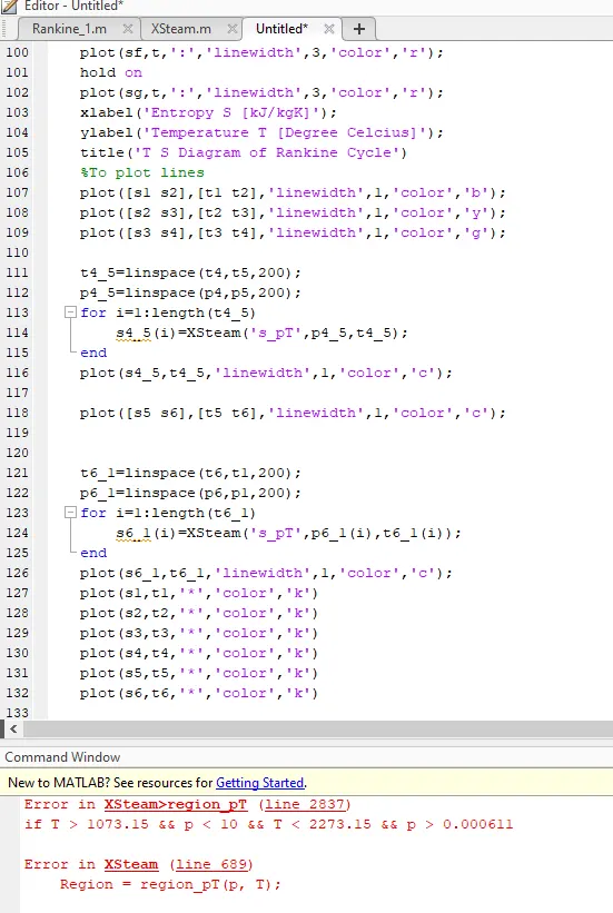
This error occured due to a typo error ,

in line 114 , p4_5(i) and t4_5(i)was written to remove the error instead of p4_5 and t4_5

2)

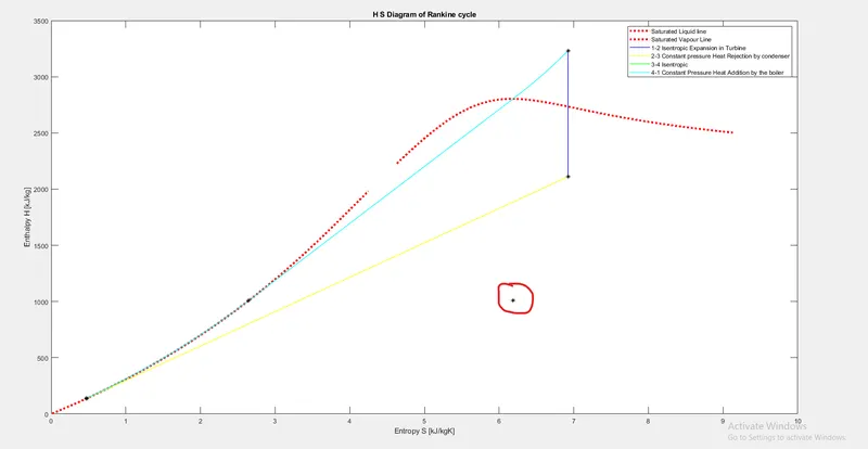
In the above diagram , state point (s6,h6) was not at the correct location .

The reason for this was that instead of saturated vapour pressure , h was obtained using saturated liquid pressure .

Hence the value was wrong . This was recified by changing the function to h6=XSteam('hV_p',p6)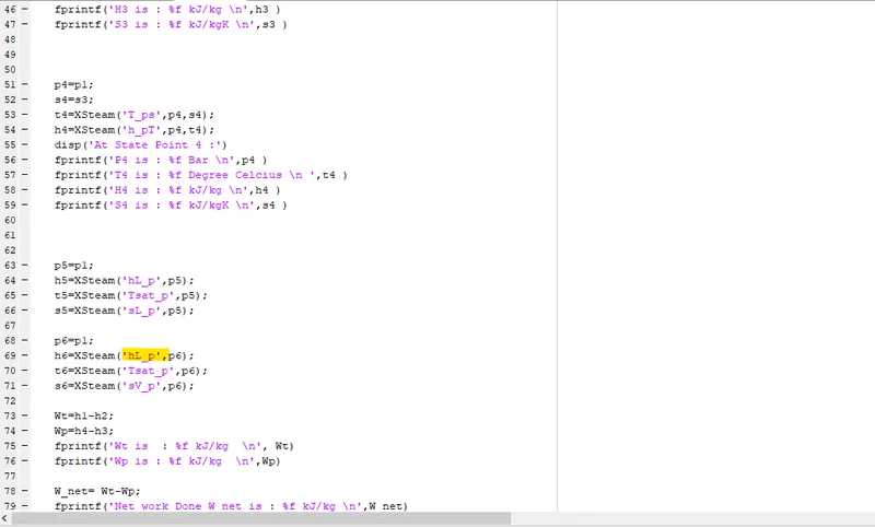

Result :

1) The program to simulate Rankine cycle was written .

2)Each state points were seperately calculated based on user input

3) TS and HS Diagrams were plotted

4) Output was obtained in required format