Rankine cycle Simulator using MATLAB

Aim: The project is to simulate 'Rankine cycle' for calculating performance of a steam turbine and to plot graphs T-s and H-S diagrams.

Objective:

The Rankine cycle is an model for predicting the performance of any steam turbine,So by using these cycle performance of steam turbine is calculated and for the easy reperesentation graphs are also plotted between T-S and H-S.

Working of Rankine cycle:

It is an basic cycle which is used for predicting the performance of steam turbine systems.In this cycle main systems are Boiler,Turbine,Condenser and Pump.By,repeating the process continuously the output as power is generated in which the steam turbine runs and converts these mechanical energy into electrical energy by boiling the water.

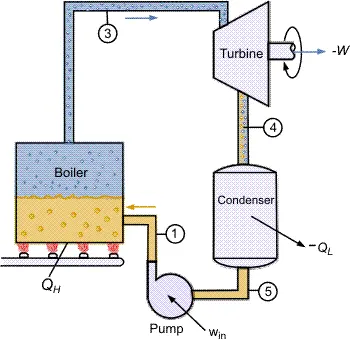
Boiler:In boiler the water is boiled by using coal and due to these steam is generated.It is at constant pressure and heat addition.

Turbine:Turbine consists of a blades and the steam which is generated in above stage is allowed to pass through these turbine and it rotates the generator then converts mechanical energy into electrical energy.It is maintained at adiabatic and expansion.

Condensor:As the steam which is left from turbine is allowed to pass through the water and converts the entire remained steam into water maintains at constant pressure and heat rejection.

Pump:The pump sucks these water and allows to enter into boiler at adiabatic and compression.

All of the above these processes are continued repeatedly for generating electricity.All the above process are reversible.The

Efficiency of these cycle can be increased by decreasing the heat added initially.It is same as carnot cycle but in a carnot cycle Liquid+steam is used for running turbines where as in these only saturated steam is used.

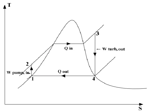
Process 1-2:Reversible,Isobaric,Head Addition

Process 2-3:Reversible,Adiabatic,Expansion

Process 3-4:Reversible,Isobaric,Heat Rejection

Process 4-1:Reversible, Adiabatic,Compression

Code Expanation:

%The basic commands used to clear all data and functions.

clear all;

close all;

clc;

%To print the name of the project.

fprintf(' RANKINE CYCLE SIMULATORn');

%To print next line.

%fprintf(' n');

%To print the process that occurs in a cycle.

fprintf('1-2 is Isentropic Expansion in the Turbinen')

fprintf('2-3 is Const Pressure Heat Rejection by the Condensern');

fprintf('3-4 is Isentropic Compression in the Pumpn');

fprintf('4-1 is Const Pressure Heat Addition by the Boilern');

%The inputs to get from a user.

P1=input('Enter the pressure at the Turbine Inlet (in bar): ');

T1=input('Enter the Temperature at the Turbine Inlet (in Degree Celsius): ');

P2=input('Enter the Pressure at the Condensor (in bar): ');

%To open and read the data from a file.

x=fopen('XSteam.m','r');

%To get enthalpy and entropy values from data file.

H1=XSteam('h_pT',P1,T1);

S1=XSteam('s_pT',P1,T1);

%During isentropically the enthalpies are same.

S2=S1;

%The values for plotting point 2 steam values.

sf2=XSteam('sL_p',P2);

sg2=XSteam('sV_p',P2);

hf2=XSteam('hL_p',P2);

hg2=XSteam('hV_p',P2);

%To find temperature at point 2.

T2=XSteam('Tsat_p',P2);

%steam value at second point.

x2=((S2-sf2)/(sg2-sf2));

H2=hf2+(x2*(hg2-hf2));

%The pressure is constant during isobaric process.

P3=P2;

%The temperature at point3.

T3=XSteam('Tsat_p',P3);

S3=XSteam('sL_p',P3);

H3=XSteam('hL_p',P3);

%Calculating the values of cp and cv.

cp=XSteam('cpL_p',P3);

cv=XSteam('cvL_p',P3);

gamma=(cp/cv);

%During isobaric process.

P4=P1;

%During isentropically.

S4=S3;

H4=XSteam('h_ps',P4,S4);

%Formula for calculating temperature at point4.

T4=T3*((P4/P3)^((gamma-1)/gamma));

%Work output of turbine.

Wt=H1-H2;

%Work done by pump.

Wp=H4-H3;

%net work done.

W_net=Wt-Wp;

%The heat supplied for heating boiler.

Q_in=H1-H2;

%The heat rejected from condenser.

Q_out=H4-H3;

%The efficiency for Rankine cycle.

n=W_netQ_in;

SSC=3600/W_net;

%Back work ratio

BWR=Q_in/Q_out;

T5=XSteam('Tsat_p',P1);

T6=T5;

S5=XSteam('sL_p',P1);

S6=XSteam('sV_p',P1);

H5=XSteam('hL_p',P1);

H6=XSteam('hV_p',P1);

%To plot graph for Entropy vs temperature.

figure(1);

Temp_1=linspace(T5,T1,500);

%The for loop is used.

for i=1:length(Temp_1)

S(i)=XSteam('s_pt',P1,Temp_1(i));

end

hold on;

%Plotting the graph by giving values.

plot([S1 S2 S3 S4 S5 S6 S],[T1 T2 T3 T4 T5 T6 Temp_1],'linewidth',3,'color','b');

axis([0 10 0 430]);

text(S1,T1,'1','FontSize',10);

text(S2,T2,'2','FontSize',10);

text(S3,T3,'3','FontSize',10,'verticalalignment','top');

text(S4,T4,'4','FontSize',10,'verticalalignment','bottom','horizontalalignment','right');

text(S5,T5,'5','FontSize',10,'verticalalignment','top');

text(S6,T6,'6','FontSize',10,'verticalalignment','top','horizontalalignment','right');

Temp_2=linspace(0,T1,500);

for j=1:length(Temp_2)

sl(j)=XSteam('sL_T',Temp_2(j));

sv(j)=XSteam('sV_T',Temp_2(j));

hl(j)=XSteam('hL_T',Temp_2(j));

hv(j)=XSteam('hV_T',Temp_2(j));

end

plot(sl,Temp_2,'linewidth',2,'color','g');

plot(sv,Temp_2,'linewidth',2,'color','g');

xlabel('Entropy in (kJ/KgK)');

ylabel('Temperature in degree(c)');

title('Entropy vs Temperature');

%To plot graph for Enthalpy vs Entropy.

figure(2);

hold on

%Values for plotting graph.

plot([S1 S2 S3 S4 S1],[H1 H2 H3 H4 H1],'linewidth',4,'color','b');

axis([0 10 -100 3500]);

text(S1,H1,'1','FontSize',10);

text(S2,H2,'2','FontSize',10);

text(S3,H3,'3','FontSize',10,'verticalalignment','top','horizontalalignment','left');

text(S4,H4,'4','FontSize',10,'verticalalignment','bottom','horizontalalignment','right');

plot(sv,hv,'linewidth',2,'color','g');

plot(sl,hl,'linewidth',2,'color','g');

xlabel('Entropy in (kJ/KgK)');

ylabel('Enthalpy in (kJ/Kg)');

%printing the results.

fprintf(' Resultsn');

%The state point1. %The state point4.

fprintf('n At State Point 1: At State Point 4: n');

fprintf('P1 is :%f in Bar P4 is :%f in Bar n',P1,P4);

fprintf('T1 is :%f in Deg Celsius T4 is :%f in Deg Celsius n',T1,T4);

fprintf('H1 is :%f in kJ/Kg H4 is :%f in kJ/Kg n',H1,H4);

fprintf('S1 is :%f in kJ/KgK S4 is :%f in kJ/KgK n',S1,S4)

%The state point2. %To print the outputs for Rankine cycle.

fprintf('n At State Point 2: Wt : %f in KJ/Kg n',Wt);

fprintf('P2 is :%f in Bar Wp :%f in KJ/Kg n',P2,Wp);

fprintf('T2 is :%f in Deg Celsius Wnet :%f in KJ/Kg n',T2,W_net);

fprintf('H2 is :%f in kJ/Kg Ntherm :%f in percent n',H2,n);

fprintf('S2 is :%f in kJ/KgK SSC :%f in Kg/KWh n',S2,SSC);

fprintf('x2 is :%f BWR :%f n',x2,BWR);

%The state point4.

fprintf('n At State Point 3: n');

fprintf('P3 is :%f in Bar n',P3);

fprintf('T3 is :%f in Deg Celsius n',T3);

fprintf('H3 is :%f in kJ/Kg n',H3);

fprintf('S3 is :%f in kJ/KgK n',S3);

Errors:

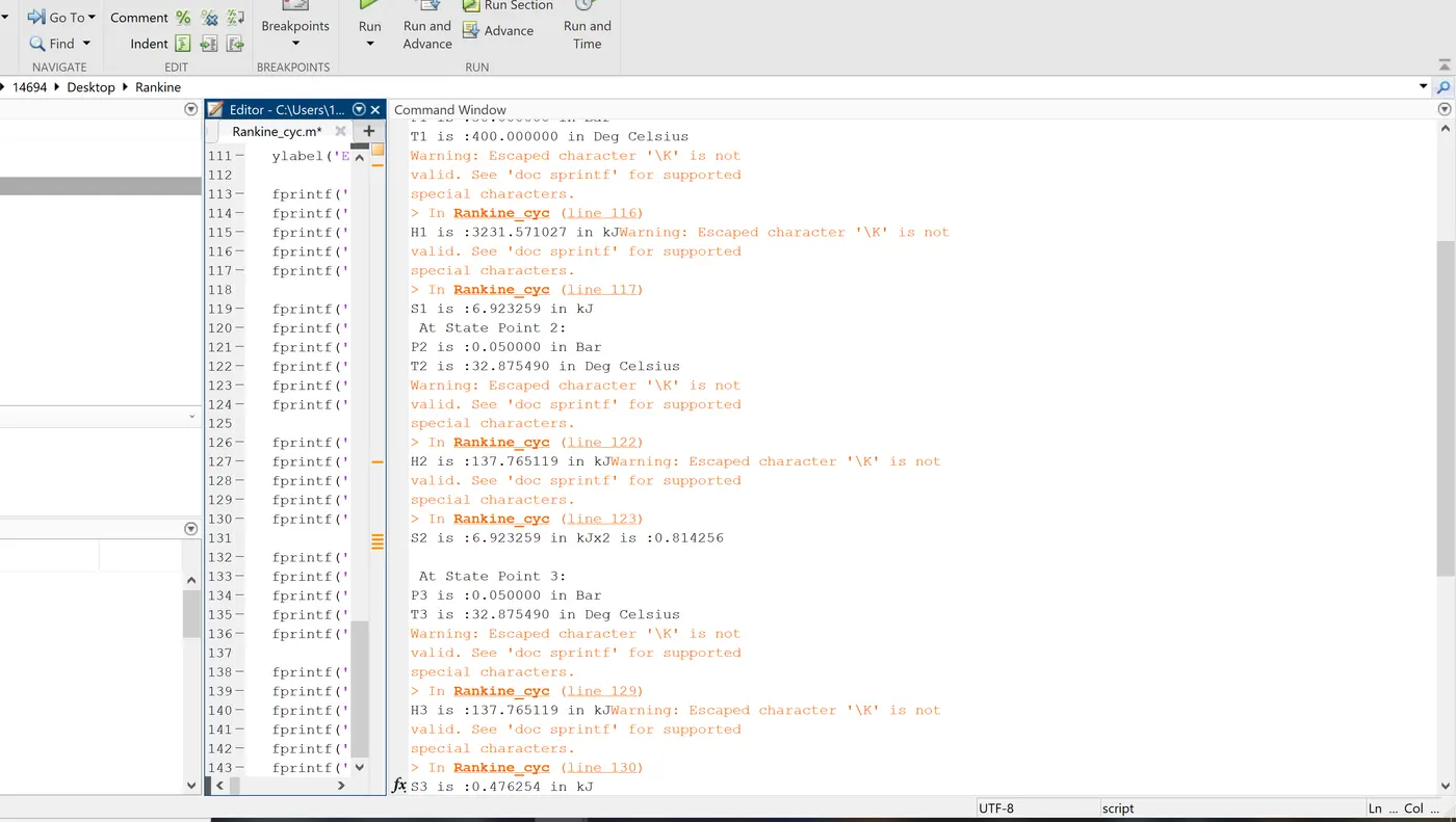
While running program many errors has been faced,but all of them has rectified easily but these error is easy determining of solution becomes difficult.

Steps taken to solve errors:

1.I have gone through some matworks documentation.

https://www.mathworks.com/help/matlabgrader/ug/view-your-solutions.html

2.Online tutorials for functions.

3.Finally,by reading matlab documentation errors are solved.

Solution:

for representing 'kilograms' used 'k' as representing 'kJ/kg'.But instead of these unfortunately used 'kJkg' then it takes to some function and shows as error.

Correct format:kJ/kg

Wrong format:kJkg

Step-wise explanation:

1. Initially start with basic functions to clear running of other programs and to clear screen.
2. The name of the project is printed by using the command ‘fprintf’.
3. Then,the functions of each process is printed from 1 to 4.
4. Getting the inputs from users as initial conditions as inlet pressure and temperature of turbine and pressure of condenser by using function ‘input’.
5. The data file is open and read the values by using function ‘fopen’.
6. The initial values of enthalpy and entropy are read from file.
7. During isentropically the entropies at state1 and state2 are equal,and values at steam conditions are read and printed from file.
8. The temperature at state2 is obtained by using formula and steam values are read.
9. During isobaric the pressure at state2 and state3 are equal.
10. The all values at state3 are calculated.
11. The temperature at state4 is calculated and all other values are obtained.
12. The work done by turbine and work given to the pump are to be calculated by using enthalpies.
13. The efficiency of cycle is calculated and back work ratio is obtained.
14. The temperature is divided into 500 parts between t5 and t1 points.
15. The ‘for’ loop is used for calculating all the values of temperatures at same temperature for plotting graphs.
16. The ‘plot’ function is used for plotting the values of entropy and temperature.
17. For plotting next graph between entropy and enthalpy the values for plotting graphs are obtained.
18. The temperature is divided in to 500 parts from initial value and t1.
19. The values of enthalpy and entropy at all different temperatures is obtained for plotting graphs.
20. The ‘plot’ function is used for plotting graphs for the values of entropy and enthalpy.
21. The results is printed at all points.
22. The list of five state points with all values are printed in the command window.
23. The values of work done,Net work,Efficiency and BWR are calculated and displayed.

Conclusion:

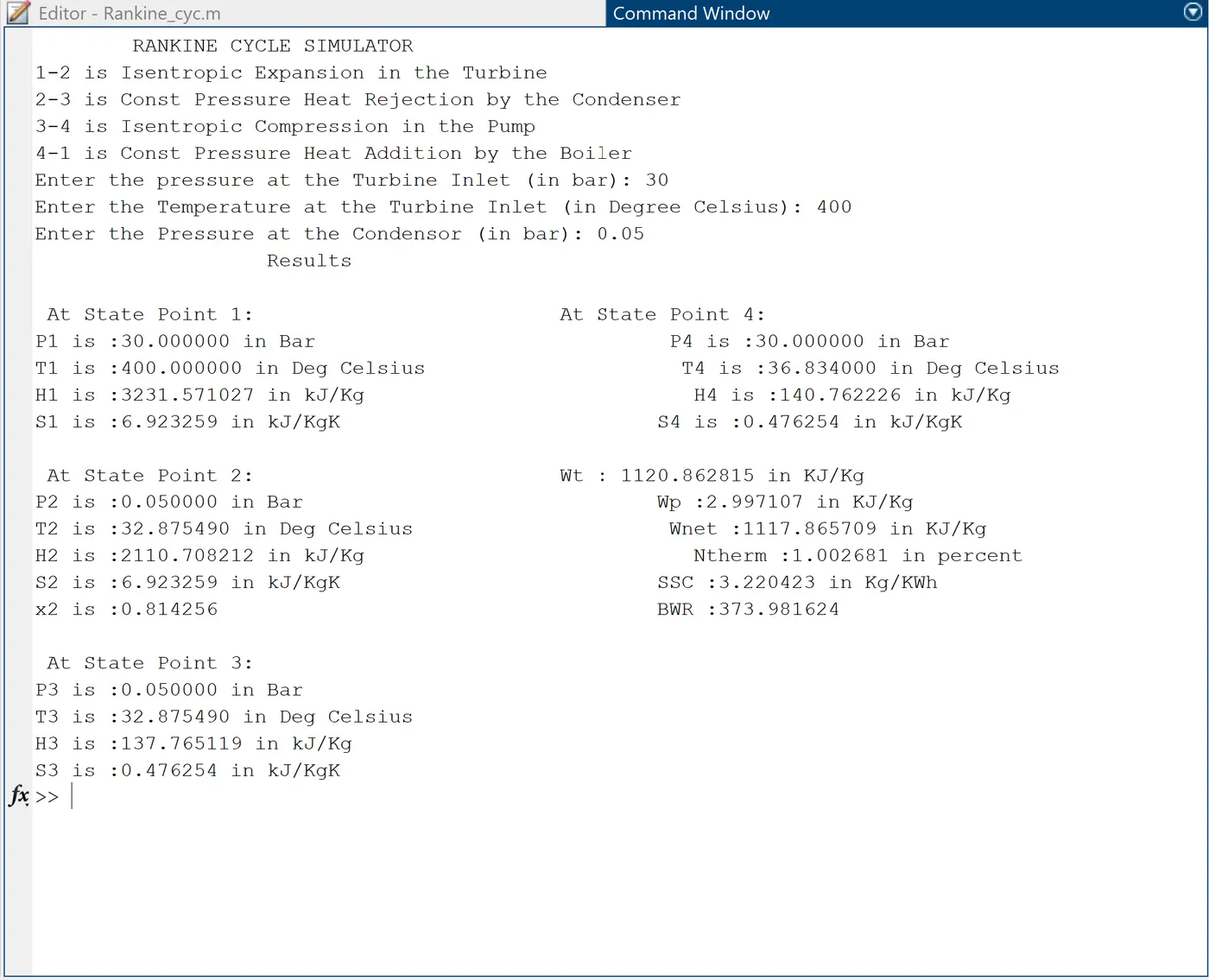
I have solved above problem by using the method same as problems solved in college days.By using the basic formulaes and the step by step solving method by extracting data values from file 'Xsteam'.Thus the graphs for T-S and H-S are plotted.

Plots:

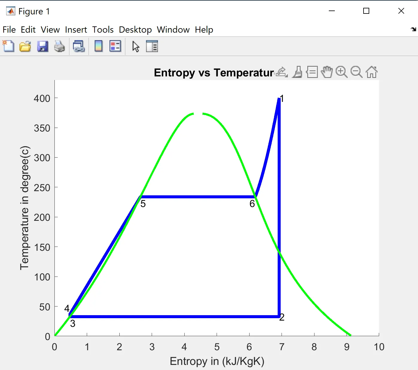
The above graph is between Entropy and Temperature.

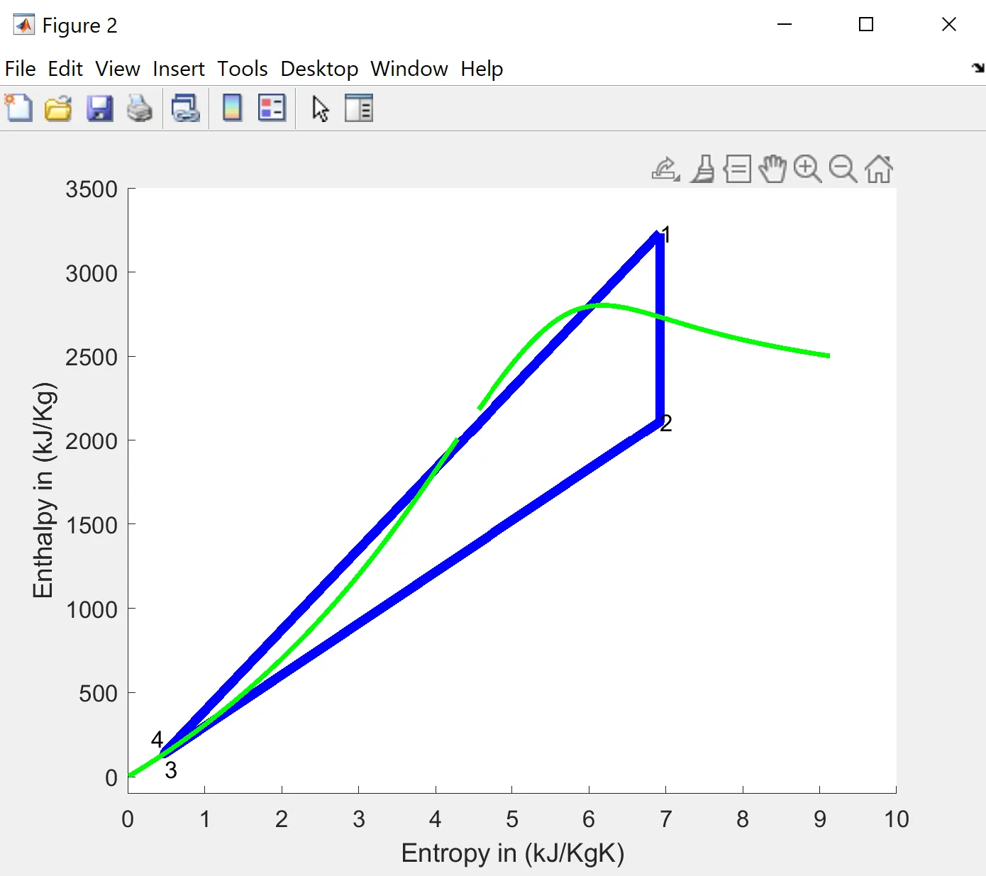
The above graph is between Entropy and Enthalpy.

Results:

1)The work output from turbine:1.1209

2)The work done on the pump: 2.997107 in KJ/Kg

3)Efficiency of cycle: 1.002681 in percent

4)The BackWorkRatio: 373.981624

5)The Network output: 1117.865709 in KJ/Kg

6)The BWR :373.981624

Reference:

1.http://home.iitk.ac.in/~suller/lectures/lec29.htm

2.https://www.learnthermo.com/T1-tutorial/ch09/lesson-B/pg07.php

3.http://www.thermopedia.com/content/1072/

4.http://www.thermopedia.com/authors/447/

%program for 'Rankine cycle Simulator' in matlab.
clear all;
close all;
clc;

fprintf('        RANKINE CYCLE SIMULATORn');
%fprintf(' n');
fprintf('1-2 is Isentropic Expansion in the Turbinen')
fprintf('2-3 is Const Pressure Heat Rejection by the Condensern');
fprintf('3-4 is Isentropic Compression in the Pumpn');
fprintf('4-1 is Const Pressure Heat Addition by the Boilern');

P1=input('Enter the pressure at the Turbine Inlet (in bar): ');
T1=input('Enter the Temperature at the Turbine Inlet (in Degree Celsius): ');
P2=input('Enter the Pressure at the Condensor (in bar): ');
x=fopen('XSteam.m','r');

H1=XSteam('h_pT',P1,T1);
S1=XSteam('s_pT',P1,T1);

S2=S1;
sf2=XSteam('sL_p',P2);
sg2=XSteam('sV_p',P2);
hf2=XSteam('hL_p',P2);
hg2=XSteam('hV_p',P2);

T2=XSteam('Tsat_p',P2);
x2=((S2-sf2)/(sg2-sf2));

H2=hf2+(x2*(hg2-hf2));

P3=P2;
T3=XSteam('Tsat_p',P3);
S3=XSteam('sL_p',P3);
H3=XSteam('hL_p',P3);

cp=XSteam('cpL_p',P3);
cv=XSteam('cvL_p',P3);
gamma=(cp/cv);

P4=P1;
S4=S3;
H4=XSteam('h_ps',P4,S4);
T4=T3*((P4/P3)^((gamma-1)/gamma));
Wt=H1-H2;
Wp=H4-H3;
W_net=Wt-Wp;

Q_in=H1-H2;
Q_out=H4-H3;

n=W_netQ_in;
%n_percent=n*100;

SSC=3600/W_net;

BWR=Q_in/Q_out;

T5=XSteam('Tsat_p',P1);
T6=T5;
S5=XSteam('sL_p',P1);
S6=XSteam('sV_p',P1);
H5=XSteam('hL_p',P1);
H6=XSteam('hV_p',P1);


figure(1);
Temp_1=linspace(T5,T1,500);

for i=1:length(Temp_1)
    S(i)=XSteam('s_pt',P1,Temp_1(i));
end

hold on;

plot([S1 S2 S3 S4 S5 S6 S],[T1 T2 T3 T4 T5 T6 Temp_1],'linewidth',3,'color','b');
axis([0 10 0 430]);
text(S1,T1,'1','FontSize',10);
text(S2,T2,'2','FontSize',10);
text(S3,T3,'3','FontSize',10,'verticalalignment','top');
text(S4,T4,'4','FontSize',10,'verticalalignment','bottom','horizontalalignment','right');
text(S5,T5,'5','FontSize',10,'verticalalignment','top');
text(S6,T6,'6','FontSize',10,'verticalalignment','top','horizontalalignment','right');


Temp_2=linspace(0,T1,500);
for j=1:length(Temp_2)
    sl(j)=XSteam('sL_T',Temp_2(j));
    sv(j)=XSteam('sV_T',Temp_2(j));
    hl(j)=XSteam('hL_T',Temp_2(j));
    hv(j)=XSteam('hV_T',Temp_2(j));
end

plot(sl,Temp_2,'linewidth',2,'color','g');
plot(sv,Temp_2,'linewidth',2,'color','g');
xlabel('Entropy in (kJ/KgK)');
ylabel('Temperature in degree(c)');
title('Entropy vs Temperature');

figure(2);
hold on
plot([S1 S2 S3 S4 S1],[H1 H2 H3 H4 H1],'linewidth',4,'color','b');
axis([0 10 -100 3500]);
text(S1,H1,'1','FontSize',10);
text(S2,H2,'2','FontSize',10);
text(S3,H3,'3','FontSize',10,'verticalalignment','top','horizontalalignment','left');
text(S4,H4,'4','FontSize',10,'verticalalignment','bottom','horizontalalignment','right');

plot(sv,hv,'linewidth',2,'color','g');
plot(sl,hl,'linewidth',2,'color','g');
xlabel('Entropy in (kJ/KgK)');
ylabel('Enthalpy in (kJ/Kg)');
fprintf('                   Resultsn');

fprintf('n At State Point 1:                         At State Point 4: n');
fprintf('P1 is :%f in Bar                             P4 is :%f in Bar n',P1,P4);
fprintf('T1 is :%f in Deg Celsius                     T4 is :%f in Deg Celsius n',T1,T4);
fprintf('H1 is :%f in kJ/Kg                           H4 is :%f in kJ/Kg n',H1,H4);
fprintf('S1 is :%f in kJ/KgK                          S4 is :%f in kJ/KgK n',S1,S4)

fprintf('n At State Point 2:                         Wt : %f in KJ/Kg n',Wt);
fprintf('P2 is :%f in Bar                             Wp :%f in KJ/Kg n',P2,Wp);  
fprintf('T2 is :%f in Deg Celsius                     Wnet :%f in KJ/Kg n',T2,W_net);
fprintf('H2 is :%f in kJ/Kg                           Ntherm :%f in percent n',H2,n);
fprintf('S2 is :%f in kJ/KgK                          SSC :%f in Kg/KWh n',S2,SSC);
fprintf('x2 is :%f                                    BWR :%f n',x2,BWR);

fprintf('n At State Point 3: n');
fprintf('P3 is :%f in Bar n',P3);
fprintf('T3 is :%f in Deg Celsius n',T3);
fprintf('H3 is :%f in kJ/Kg n',H3);
fprintf('S3 is :%f in kJ/KgK n',S3);