Parsing NASA thermodynamic data using MATLAB

Aim:To extract the data from file using matlab functions and calculating enthalpy,entropy and specific heats of all species then plotting graphs between different species at different temperatures.

FILE PARSING:

It is a process of extracting data from required files and using these data for performing operations like graphs, calculations etc.

FILE FORMATS:

.txt,excel,.docx,data.

FUNCTIONS USED:

1. “fopen” function:It is used to open file.
2. “fgetl” function:for reading a line in a file.
3. “strsplit” function:To split a function.
4. “str2num” function:To convert strings to numbers.
5. “findstr” function: for finding particulat string.
6. “mkdir” function:To create a folder.
7. “linspace” function:For dividing two values at a particular spaces.
8. “plot” function:To plot graphs.
9. “title” function:To give title to graph.
10. “cd” function:To change directory for current folder.
11. “sprint” function:To read inside text.
12. “fclose” function:To close the reading of file.

Logic used for reading data line by line:

1. At first ‘fgetl’ is used to read first line.
2. By same pattern other lines are to be readed by ‘fgetl’.
3. But the line which has co-efficients are to be separated and the each co-efficients are to be read and declared to a variable.
4. For doing these we should split function by using something.
5. So,I chose an variable(‘E‘)which can be used to separate these can be done by using ‘findstr’.
6. Then,all these co-efficients are separated and declared to a variables.
7. By using ‘str2num’ the strings are to be converted in to numbers.

OBJECTIVE:

Main objective of the project is to read data line by line from file and separate the coefficients from lines and declare these to variables.To find entropy,enthalpy and specific heat required formulas are to be selected then for calculating these formulas the required co-efficients are to be used.For different species all these are to be calculated and plots are calculated for each species between enthalpy,entropy,specific heat and temperatures.The molecular weights for all species are calculated by using required formulas.

Explanation of Complete code Logic:

1. Initially,the commands like clearall,closeall and clc are used.
2. I used ‘fopen’ function to open the data file.
3. Then the next line is read by using function ‘fgetl’.
4. The temperatures are read using function ‘fgetl’ and declared these line to a variable ‘Global_temp’.
5. But in this line there are many temperatures,so reading of each temperature is important for ‘parsing data’.
6. The function ‘strsplit’ is used to separate these temperatures.For separating these temperatures are done through selecting the space(‘ ‘) between them.
7. Then each temperature is declared to each variable as follows Global_max_temp,Global_min_temp and Global_mid_temp.
8. The next three lines which are header files which is not useful,but they are store in variable ‘header’ using function ‘fgetl’.
9. The number of species are 53,so to execute the program for 53 times the loop ‘if’ is used.
10. The next line which includes species name,Local temperature are read by using ‘fgetl’ function.
11. The first column is declared to ‘Name of the species’.
12. The next four columns are not useful,at starting from sixth column the temperatures are started these three temperatures are declared to a variables which are local temperatures as follows Local_max_temp,Local_min_temp and Local_mid_temp.
13. The next line is read and stored as it contains the co-efficients which are to be separated and declared to a particular variables.
14. For separating these co-efficients the logic followed is by finding the positions of a variable which is included in each co-efficients.The commom variable which is found in each co-efficient is ‘E’.
15. The positions of variable is noted at each co-efficients and then by adding the number of spaces for each co-efficient is calculated and these converted to number by using function ‘str2num’.
16. By,these way the 14 co-efficients are read line by line by adding the positions and declaring the above co-efficient positions all co-efficients are declared to 16 different variables.
17. In these initial seven co-efficients are at high temperatures and remaining seven co-efficients are at low temperatures.
18. Then the local_temperature is declared for dividing Local_max_temperatures and Local_min_temperatures in to thousand parts by using function ‘linspace’.
19. Value of ‘R’ which is universal constant is declared.
20. The variable ‘j’ is declared for storing the length of local_temperature.
21. The ‘if’ loop is used for using the low temperatre co-efficients at one condition and high temperature co-efficients at other condition.
22. If the local temperature is greater than or equal to local_mid_temp the high co-efficients are used for calculating the formula Enthalpy,entropy and specific heat.
23. The loop ‘else’ is used if the above conditions are violated then low temperature co-efficients are used for calculating formulas.
24. Then the oop is ‘end’.
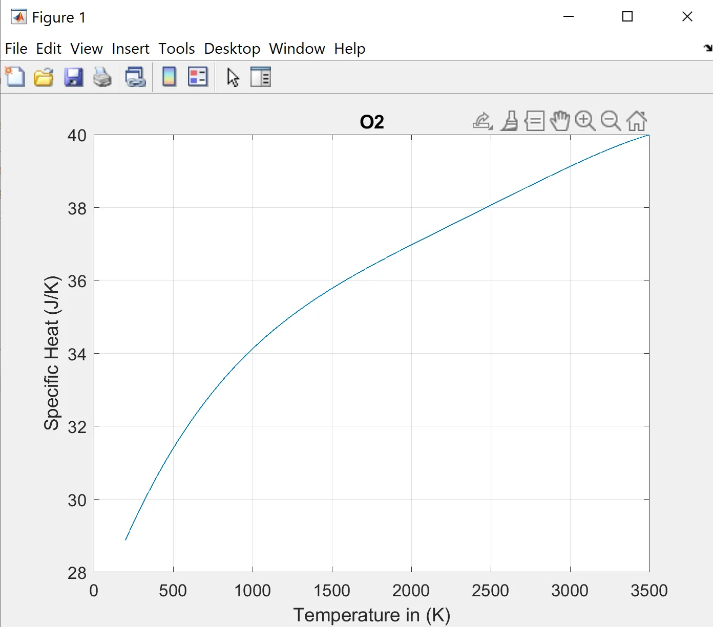
25. The ‘figure(1)’ is plotted between local_temp and cp.
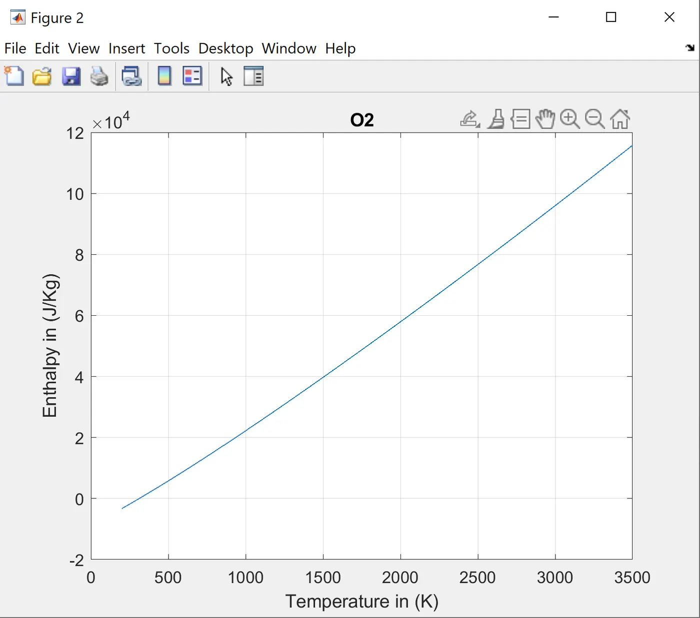
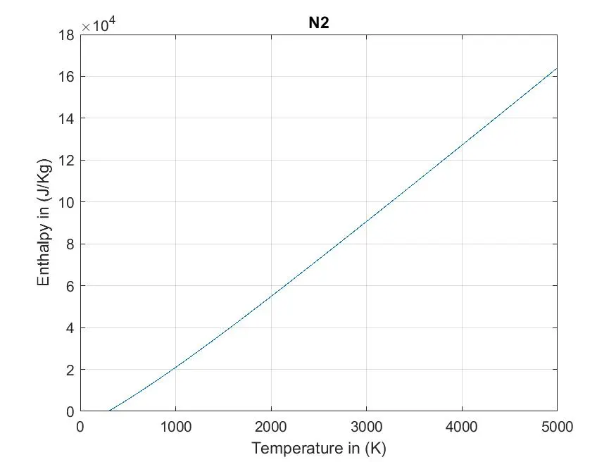
26. The ‘figure(2)’ is plotted between local_temp and H.
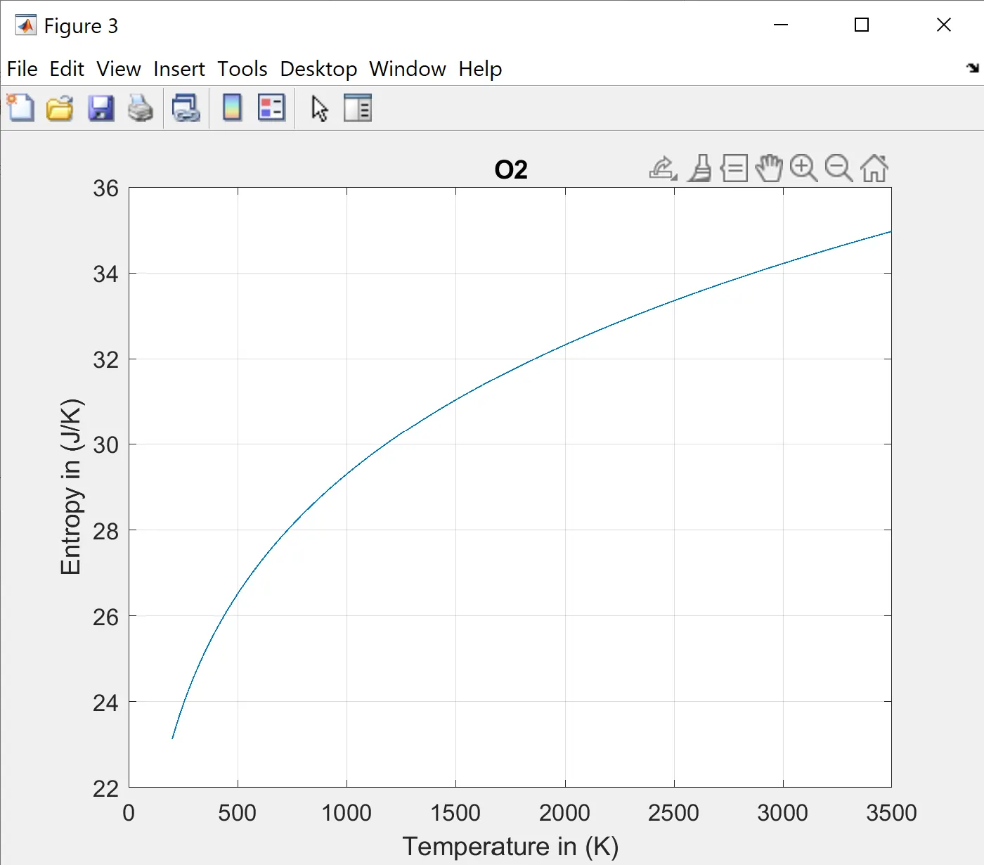
27. The ‘figure(3)’ is plotted between local_temp and S.
28. Then by using ‘cd’ function the directory is changed and the graphs of each species are stored in that directory.
29. The elements and Atomic_wts are declared for species.
30. The for loop is used for calculating the molecular weight of each species and stored to the variable ‘mol_mass’.
31. The ‘for’ loop is end.

The file is closed by usig functon ‘fclose’.

Errors Faced:

FIRST:

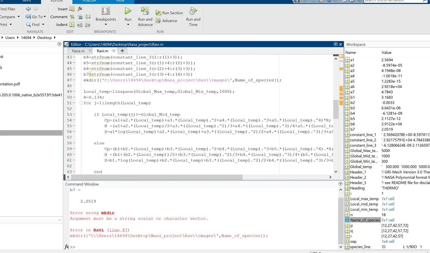
I have faced errors during the usage of function 'mkdir'.I have overcome these errors by understanding the function usage and it's declarations.

SOLUTION:

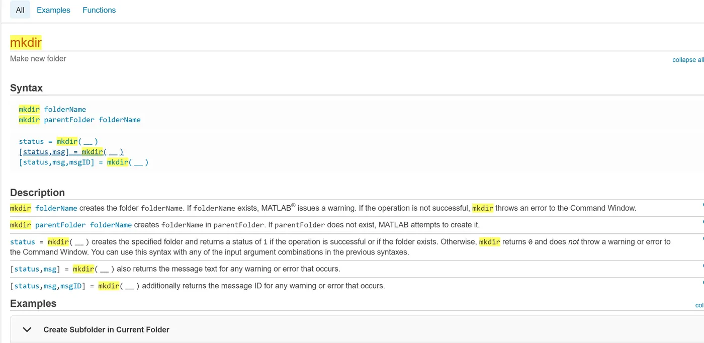
SECOND:

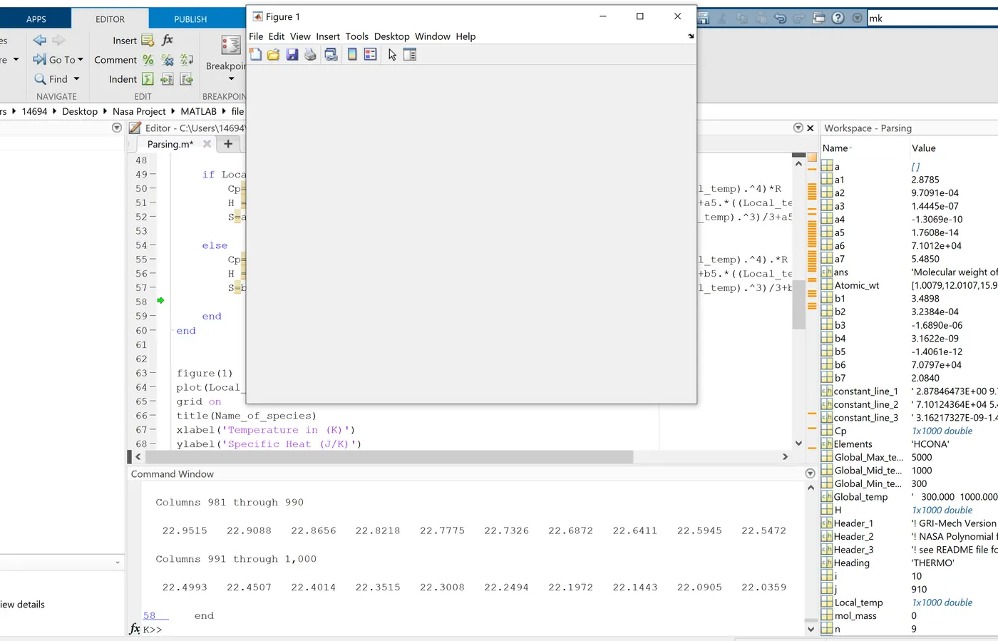
The graphs are obtained without readings as my THERMO data file is saved as ".txt" format then it has been converted to ".dat" format for extracting the data in a easy way.

SOLUTION:

By,going through some readings then I have learnt to convert file format in to '.dat' format.

Steps taken to overcome these Errors:

1.At first gone through the tutorials in skill-lync and understanding an logic behind these data extracting.

2.Matlab documentation.

3.https://youtu.be/OZCGEbF4Lbs

4.Then,finally by skill-lync support the errors are solved.

Step-Wise Expanation of code:

1.These are the commands used initially to clear the data.

clear all;

close all;

clc;

2.To open data file which is to be extracted.

n=fopen('Nasadata.txt','r');

3.It is an heading.

Heading=fgetl(n);

4.The temperatures are extracted and declared to a variable.

Global_temp=fgetl(n);

5.The temperatures are being separated.

sep=strsplit(Global_temp,' ');

6.The temperatures are declared to different variables.

Global_Min_temp=str2num(sep{2});

Global_Mid_temp=str2num(sep{3});

Global_Max_temp=str2num(sep{4});

7.The headers are read and declared.

Header_1=fgetl(n);

Header_2=fgetl(n);

Header_3=fgetl(n);

8.The ‘for’ loop is used for doing operations for fifty three times.

for i=1:53

9.The species line is read and declared to a variable.

species_line=fgetl(n);

10.To get particular name of species the line is splitted.

z=strsplit(species_line,' ');

11.Particular name is species is declared.

Name_of_species=z{1};

12.The local temperatures are declare to different variables.

Local_max_temp=str2num(z{6});

Local_mid_temp=str2num(z{7});

Local_min_temp=str2num(z{8});

13.The line of co-efficients.

constant_line_1=fgetl(n);

14.The string is separated by using the positions of variable ‘E’.

p=findstr(constant_line_1,'E');

15.By calculating the exact positions of these variable the co-efficients are read and declared to different variables.And by using the position of above co-efficient the next co-efficients can be calculated by adding it’s positions.In,this way the seventeen co-efficients are declared.

a1=str2num(constant_line_1(1:p(1)+3));

a2=str2num(constant_line_1(p(1)+4:p(2)+3));

a3=str2num(constant_line_1(p(2)+4:p(3)+3));

a4=str2num(constant_line_1(p(3)+4:p(4)+3));

a5=str2num(constant_line_1(p(4)+4:p(5)+3));

constant_line_2=fgetl(n);

q=findstr(constant_line_2,'E');

a6=str2num(constant_line_2(1:q(1)+3));

a7=str2num(constant_line_2(q(1)+4:q(2)+3));

b1=str2num(constant_line_2(q(2)+4:q(3)+3));

b2=str2num(constant_line_2(q(3)+4:q(4)+3));

b3=str2num(constant_line_2(q(4)+4:q(5)+3));

constant_line_3=fgetl(n);

r=findstr(constant_line_3,'E');

b4=str2num(constant_line_3(1:r(1)+3));

b5=str2num(constant_line_3(r(1)+4:r(2)+3));

b6=str2num(constant_line_3(r(2)+4:r(3)+3));

b7=str2num(constant_line_3(r(3)+4:r(4)+3))

16.To create file in particular folder.

mkdir('Name_of_species');

17.The max temp and min temp are divided in to 1000 parts.

Local_temp=linspace(Local_max_temp,Local_min_temp,1000);

R=8.134;

18.The for loop is executed and the length of temperature is noted.

for j=1:length(Local_temp)

19.The ‘if’ condition is used as to calculate formula by using starting seven co-efficients which are at high temperatures.

if Local_temp(j)>=Local_mid_temp

Cp=(a1+a2.*(Local_temp)+a3.*(Local_temp).^2+a4.*(Local_temp).^3+a5.*(Local_temp).^4)*R;

H =(a1+a2.*(Local_temp)/2+a3.*((Local_temp).^2)/3+a4.*((Local_temp).^3)/4+a5.*((Local_temp).^4)/5).*R.*(Local_temp);

S=a1*log(Local_temp)+a2.*(Local_temp)+a3.*((Local_temp).^2)/2+a4.*((Local_temp).^3)/3+a5.*(((Local_temp).^4)/4)+a7;

20.If above condition is violated then by using ‘else’ the co-efficients at lower temperatures are used for calculating formulas.

else

Cp=(b1+b2.*(Local_temp)+b3.*(Local_temp).^2+b4.*(Local_temp).^3+b5.*(Local_temp).^4).*R;

H =(b1+b2.*(Local_temp)/2+b3.*((Local_temp).^2)/3+b4.*((Local_temp).^3)/4+b5.*((Local_temp).^4)/5).*R.*(Local_temp);

S=b1.*log(Local_temp)+b2.*(Local_temp)+b3.*((Local_temp).^2)/2+b4.*((Local_temp).^3)/3+b5.*((Local_temp).^4)/4+b7;

end

end

21.The graph is plotted between temperature and cp.

figure(1);

plot(Local_temp,Cp);

grid on;

title(Name_of_species);

xlabel('Temperature in (K)');

ylabel('Specific Heat (J/K)');

22.The graph is plotted between temperature and H.

figure(2);

plot(Local_temp,H);

grid on;

title(Name_of_species);

xlabel('Temperature in (K)');

ylabel('Enthalpy in (J/Kg)');

23.The graph is plotted between temperature and S.

figure(3);

plot(Local_temp,S);

grid on;

title(Name_of_species);

xlabel('Temperature in (K)');

ylabel('Entropy in (J/K)');

24.The directory of file is changed by using the function ‘cd’ and to save the graphs.

save=(['C:Users14694Desktopsaiimages',Name_of_species]);

cd(save);

saveas(1,'Specific Heat','jpg');

saveas(2,'Enthalpy','jpg');

saveas(3,'Entropy','jpg');

25.For calculaing the molecular weights of each species.

Elements=['H','C','O','N','A'];

Atomic_wt=[1.0079 12.0107 15.999 14.0067 39.948];

mol_mass=0;

26.The ‘for’ loop is used for reading all species.

for a=1:length(Name_of_species)

for b=1:length(Atomic_wt)

if strcmp(Name_of_species(a),Elements(b))

mol_mass=mol_mass+Atomic_wt(b);

position=b;

end

end

k=str2double(Name_of_species(a));

if n>1

mol_mass=mol_mass+Atomic_wt(position)*(n-1);

end

end

sprintf('Molecular weight of %s:%f u',Name_of_species,mol_mass);

end

27.To close the file.

fclose(n);

Results:

Species ‘H’:

Enthalpy:

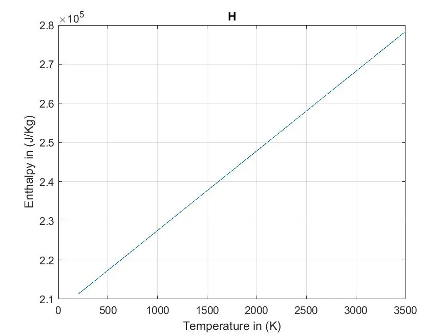
At initially the temperature starts increasing as follows these enthalpy also started increasing slightly as temperature increases.

Entropy:

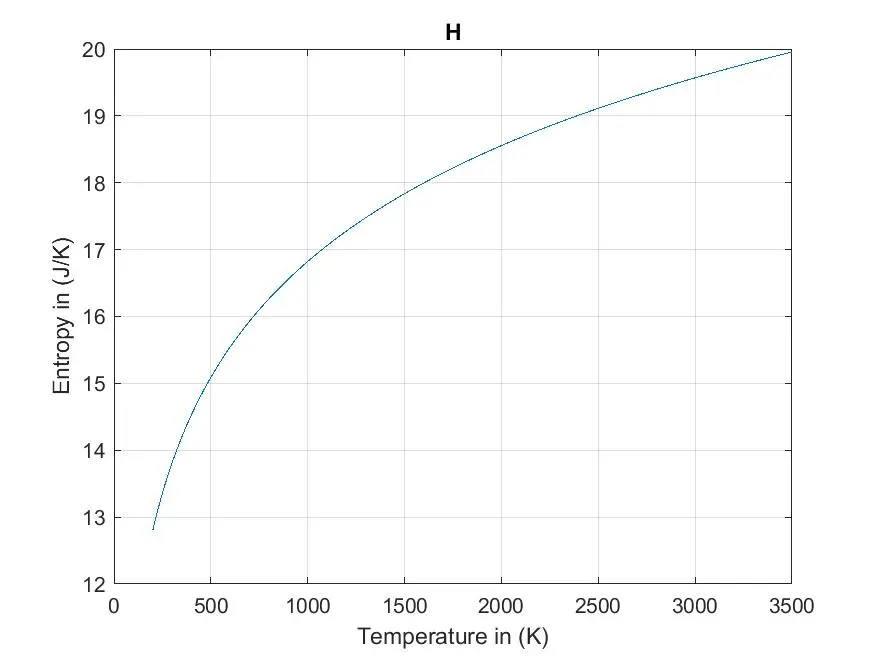
At initially both are at same point then later at small increase in Temperature the entropy increases more at final stage both are stopped at one point.

Specific heat:

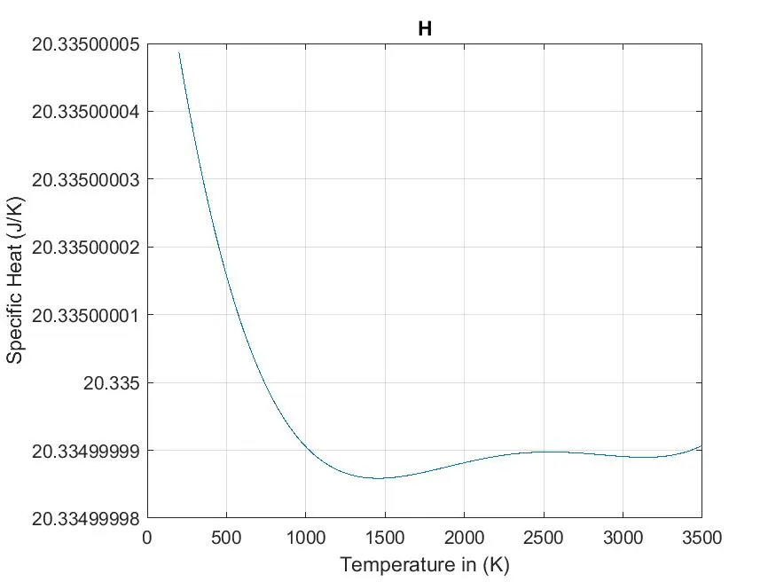
At initially the specific heat is st very high as slight increase in temperature results to more decrease in specific heat then finally the temperature is high at which specific heat is very low.

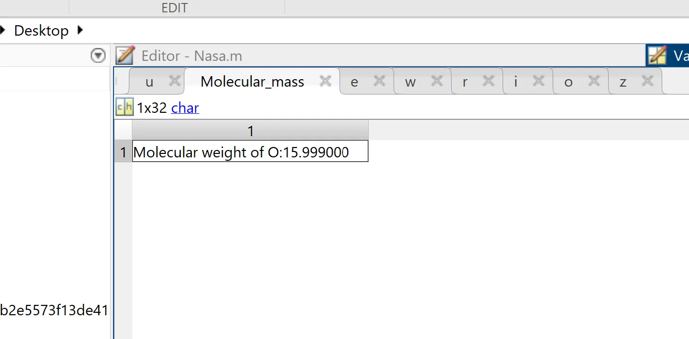
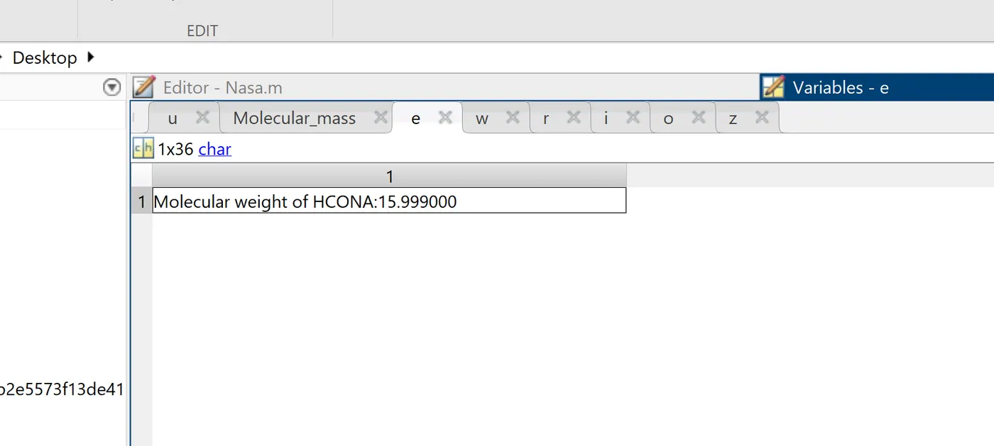
The molecular weights of different species:

CONCLUSION:

The fiftythree species are extracted and graphs are plotted for each species and these are saved in folder as species name.

The Graphs for some of the species are as follows.

Species 'O2'

Specific heat:

Enthalpy:

Entropy:

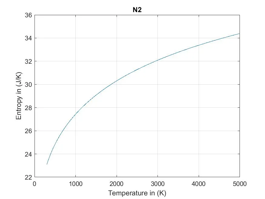
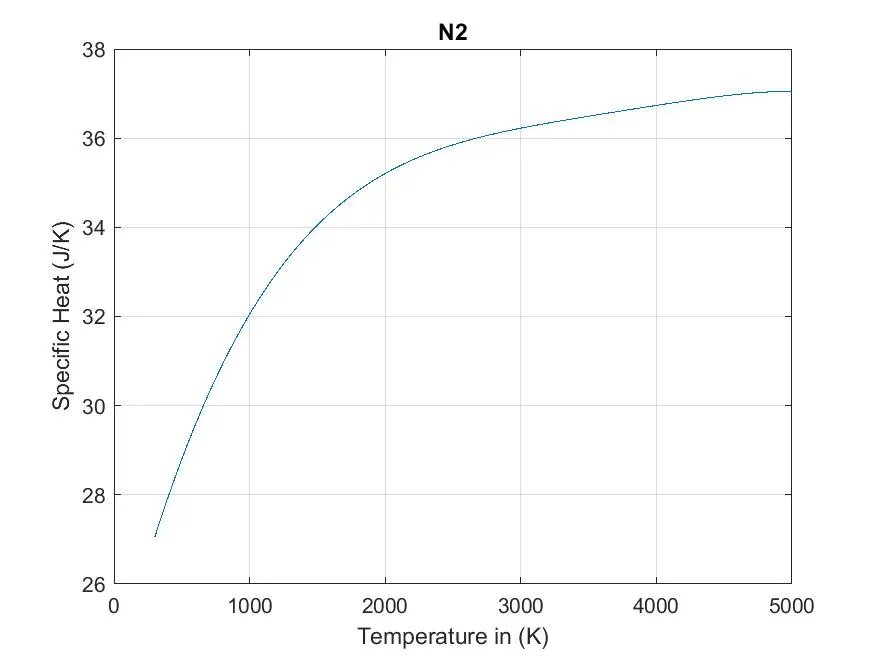
Species 'N2'

Enthalpy:

Entropy:

Specific Heat:

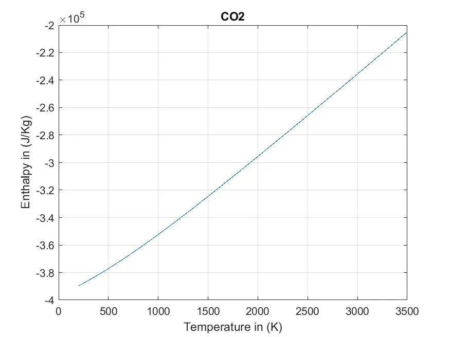
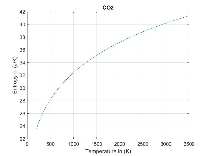
Species 'CO2'

Enthalpy:

Entropy:

Specific Heat:

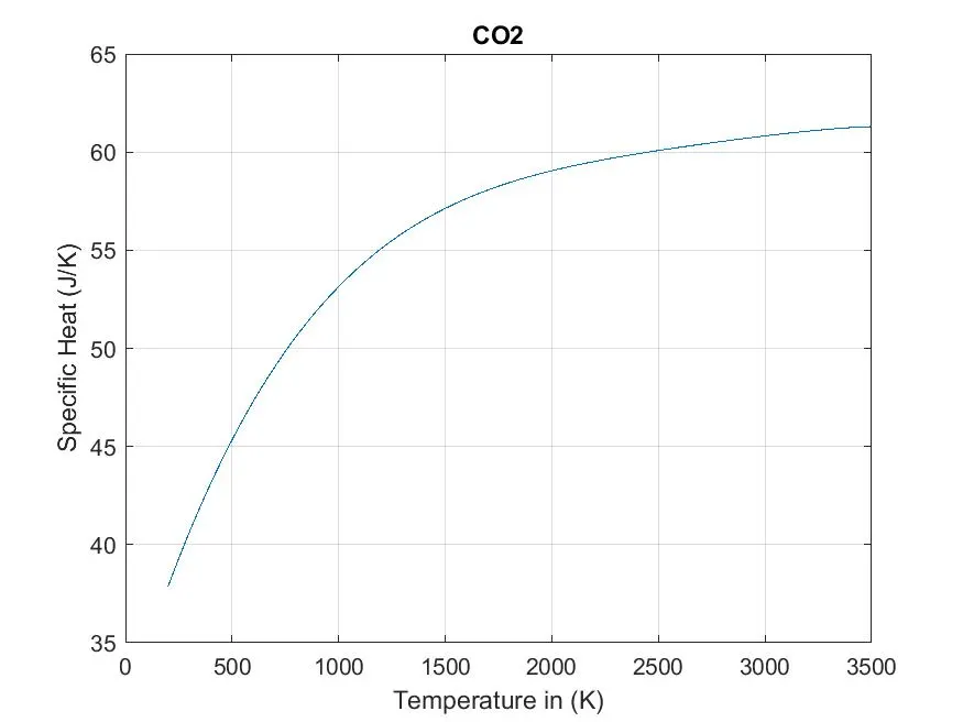
By,using the logics which are mentioned in above coding is the procces followed for extracting data by reading line by line each digit of text and then assigned all these things to variables for calculating the formulas for enthalpy,entropy and specific heat.The temperatures are assigned by dividing into parts.

And plots are plotted for fiftythree species and saved in a directory.

%Matlab program for 'Data Parsing'.
clear all;
close all;
clc;
n=fopen('THERMO.dat','r');
Heading=fgetl(n);
Global_temp=fgetl(n);
sep=strsplit(Global_temp,' ');
Global_Min_temp=str2num(sep{2});
Global_Mid_temp=str2num(sep{3});
Global_Max_temp=str2num(sep{4});
Header_1=fgetl(n);
Header_2=fgetl(n);
Header_3=fgetl(n);

for i=1:53

species_line=fgetl(n);
z=strsplit(species_line,' ');
Name_of_species=(z{1});
y=length(z);
Local_min_temp=str2double(z{y-3});
Local_max_temp=str2double(z{y-2});
Local_mid_temp=str2double(z{y-1});
t1=Local_min_temp
t2=Local_max_temp
t3=Local_mid_temp
constant_line_1=fgetl(n);
p=findstr(constant_line_1,'E');
a1=str2num(constant_line_1(1:p(1)+3));
a2=str2num(constant_line_1(p(1)+4:p(2)+3));
a3=str2num(constant_line_1(p(2)+4:p(3)+3));
a4=str2num(constant_line_1(p(3)+4:p(4)+3));
a5=str2num(constant_line_1(p(4)+4:p(5)+3));
constant_line_2=fgetl(n);
q=findstr(constant_line_2,'E');
a6=str2num(constant_line_2(1:q(1)+3));
a7=str2num(constant_line_2(q(1)+4:q(2)+3));
b1=str2num(constant_line_2(q(2)+4:q(3)+3));
b2=str2num(constant_line_2(q(3)+4:q(4)+3));
b3=str2num(constant_line_2(q(4)+4:q(5)+3));
constant_line_3=fgetl(n);
r=findstr(constant_line_3,'E');
b4=str2num(constant_line_3(1:r(1)+3));
b5=str2num(constant_line_3(r(1)+4:r(2)+3));
b6=str2num(constant_line_3(r(2)+4:r(3)+3));
b7=str2num(constant_line_3(r(3)+4:r(4)+3))
mkdir(['C:Users14694DesktopNasa_projectNasaimages',Name_of_species]);

Temp=linspace(t1,t2,1000);
R=8.134;
for j=1:length(Temp)
    
    if Temp(j)>=t3
        Cp=(a1+a2.*Temp+a3.*Temp.^2+a4.*Temp.^3+a5.*Temp.^4)*R;
        H =(a1+(a2.*Temp)/2+(a3.*Temp.^2)/3+(a4.*Temp.^3)/4+(a5.*Temp.^4)/5+(a6./Temp))*R.*Temp;
        S=a1.*log(Temp)+a2.*Temp+(a3.*Temp.^2)/2+(a4.*Temp.^3)/3+(a5.*Temp.^4)/4+a7;
        
    else
        Cp=(b1+b2.*Temp+b3.*Temp.^2+b4.*Temp.^3+b5.*Temp.^4).*R;
        H =(b1+(b2.*Temp)/2+(b3.*Temp.^2)/3+(b4.*Temp.^3)/4+(b5.*Temp.^4)/5+(b6./Temp))*R.*Temp;
        S=b1.*log(Temp)+b2.*Temp+(b3.*Temp.^2)/2+(b4.*Temp.^3)/3+(b5.*Temp.^4)/4+b7;
        
    end
end


figure(1);
plot(Temp,Cp);
grid on;
title(Name_of_species);
xlabel('Temperature in (K)');
ylabel('Specific Heat (J/K)');

figure(2);
plot(Temp,H);
grid on;
title(Name_of_species);
xlabel('Temperature in (K)');
ylabel('Enthalpy in (J/Kg)');

figure(3);
plot(Temp,S);
grid on;
title(Name_of_species);
xlabel('Temperature in (K)');
ylabel('Entropy in (J/K)');



cd=(['C:Users14694DesktopNasa_projectNasaimages',Name_of_species]);
saveas(1,'specific Heat','jpg');
saveas(2,'enthalpy','jpg');
saveas(3,'entropy','jpg');


Elements=['H','C','O','N','A'];
Atomic_wt=[1.0079 12.0107 15.999 14.0067 39.948];
mol_mass=0;
for a=1:length(Name_of_species)
    for b=1:length(Atomic_wt)
        if strcmp(Name_of_species(a),Elements(b))
            mol_mass=mol_mass+Atomic_wt(b);
            position=b;
        end
    end
    k=str2double(Name_of_species(a));
    if k>1
        mol_mass=mol_mass+Atomic_wt(position)*(k-1);
    end
end
sprintf('Molecular weight of %s:%f ',Name_of_species,mol_mass);


end
            
fclose(n);