Project 2 - Rankine cycle Simulator
Aim:
To learn the Rankine cycle and to create a Rankine Cycle Smulator using Matlab which shows all state conditions and T-S and H-S plots.
THEORY:
The Rankine cycle or Rankine Vapor Cycle is the process widely used by power plants such as coal-fired power plants or nuclear reactors. In this mechanism, a fuel is used to produce heat within a boiler, converting water into steam which then expands through a turbine producing useful work. This process was developed in 1859 by Scottish engineer William J.M. Rankine.[1] This is a thermodynamic cycle which converts heat into mechanical energy, which usually gets transformed into electricity by electrical generation.
The steps in the Rankine Cycle as shown in Figure 1 and the corresponding steps in the pressure-volume diagram (figure) are outlined below:
1. Pump: Compression of the fluid to high pressure using a pump (this takes work) (Figure : Steps 5 to 1)
2. Boiler: The compressed fluid is heated to the final temperature (which is at boiling point), therefore, a phase change occurs—from liquid to vapour. (Figure : Steps 1to 3)
3. Turbine: Expansion of the vapour in the turbine. (Figure : Steps 3 to 4)
4. Condenser: Condensation of the vapour in the condenser (where the waste heat goes to the final heat sink (the atmosphere or a large body of water (ex. lake or river). (Figure : Steps 4 to 5)
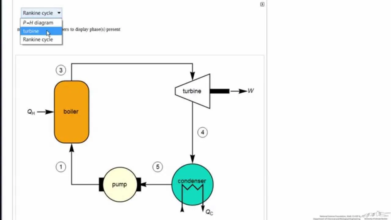
MATLAB Code:
clear all
close all
clc
%user inputs
fprintf('%75s','Rankine Cycle Simulator');
fprintf('\n \n \n')
fprintf('1-2 is Isentropic Expansion in the turbine \n');
fprintf('2-3 is Constant Pressure Heat Rejection by the Condensor \n');
fprintf('3-4 is Isentropic Compression in the Pump \n');
fprintf('4-1 is Constant Pressure Heat Addition by the Boiler \n \n');

% inputs
p1=input(' Enter the Pressure(in bar) at the inlet of the turbine(at point 1):');
t1=input(' Enter the Temperature(in degrees) at the inlet of the turbine(at point 1):');
p2=input(' Enter the pressure(in degrees) at the inlet of the Condensor(at point 2):');

%inputs to the turbin
s1 = XSteam('s_pT',p1,t1);
h1 = XSteam('h_pt',p1,t1);

% condensor inlet
s2=s1; %1-2 is an isentropic expansion process
sf2=XSteam('sL_p',p2);
sg2=XSteam('sV_p',p2);
hf2=XSteam('hL_p',p2);
hg2=XSteam('hV_p',p2);

%calculating dryness fraction
if(s2<=sg2)
    x2 = ((s2 - sf2) / (sg2-sf2));     % Dryness Fraction at state point 2
else
    x2=1;
end
h2=hf2+(x2*(hg2-hf2));

% condensor exit
p3=p2;
t3=XSteam('Tsat_p',p3);
s3=XSteam('sL_p',p3);
h3=XSteam('hL_p',p3);
v3=XSteam('vL_p',p3);
t2=t3;

% boiler inlet
p4=p1; % constant pressure heat addition
s4=s3; %isentropic compression in the pump
h4=XSteam('h_ps',p4,s4);
cp4=XSteam('Cp_ps',p4,s4);
cv4=XSteam('Cv_ps',p4,s4);
g4=(cp4/cv4);
% calculation for t4
%p4^(1-gamma)*t4^gamma=p3^(1-gamma)*t3^gamma;
t4=(t3*((p3/p4)^((1-g4)/g4)));

% calculations
% work done by the turbine
Wt=h1-h2;

% work done by the pump
Wp=h4-h3;

% net work done
W_net=Wt-Wp;

% heat added in the boiler
q_in=h1-h4;

% heat rejected in the condensor
q_out=h2-h3;

% Thermal efficiency
n= (W_net/q_in)*100

%plotting the results
figure(1)
%plotting liquid and vapour curves
t=linspace(1,t1,1000);
for i=1:length(t)
    s_l(i)=XSteam('sL_T',t(i));
end

for i=1:length(t)
    s_v(i)=XSteam('sV_T',t(i));
end
hold
plot(s_l,t,'linewidth',2,'linestyle','- -','color','r');
plot(s_v,t,'linewidth',2,'linestyle','- -','color','r');
grid on

% plotting for the work done by the tubrine(process 1-2)
plot([s1,s2],[t1,t2],'linewidth',2,'color','k')
hold on
title(' T-s Diagram of Ideal Rankine Cycle')
xlabel('Entropy(KJ/KgK)')
ylabel('Temperature(k)')

% Plotting for heat rejected in condensor (Process 2-3)
plot([s2,s3],[t2,t3],'linewidth',2,'color','k')
hold on

% Plotting for work done by the pump (Process 3-4)
plot([s3,s4],[t3,t4],'linewidth',2,'color','k')
hold on

% Plotting for heat added by the boiler(Process 4-1)
tp = XSteam('TSat_p',p4);
sp = XSteam('sL_T',tp);
plot([s4,sp],[t4,tp],'lineWidth',2,'color','k')
hold on

tq = tp;
sq = XSteam('sV_T',tq);
plot([sp,sq],[tp,tq],'lineWidth',2,'color','k')
hold on

plot([sq,s1],[tq,t1],'lineWidth',2,'color','k')
hold on

%Indicate states with numbers
text(s1,t1,' 1');
text(s2,t2,' 2');
text(s3,t3,' 3');
text(s4,t4,' 4');

%Plot for enthalpy vs entropy
figure(2)
plot([s1,s2],[h1,h2],'lineWidth',2,'color','k')
grid on
title('h-s DIAGRAM')
xlabel('Entropy(KJ/kgK)')
ylabel('Enthalpy(KJ/kg)')
hold on

plot([s2,s3],[h2,h3],'lineWidth',2,'color','k')
hold on
plot([s3,s4],[h3,h4],'lineWidth',2,'color','k')
hold on
plot([s4,s1],[h4,h1],'lineWidth',2,'color','k')

%plot for liqiuid and vapour saturation curve
t = linspace(1,t1,1000);
for j = 1:length(t)
    h_l(j) = XSteam('hL_T',t(j));
end
for j = 1:length(t)
    h_v(j) = XSteam('hV_T',t(j));
end

plot(s_l,h_l,'lineWidth',2,'color','r')
hold on
plot(s_v,h_v,'lineWidth',2,'color','r')
%Indicate states with numbers
text(s1,h1,'1');
text(s2,h2,'2');
text(s3,h3,'3');
text(s4,h4,'4');- output plot: