• Aim : optimise the stalagmite function and find the global maxima of the function.
• Theory : A genetic algorithm is an algorithm that imitates the process of Natural Selection. Natural selection is a central concept of evolution: some organism has traits that will make it more likely that the organism survives long enough to reproduce. That way, it is likely that these traits will be passed on to the next generation. This has also been called survival of the fittest. This algorithm reflects the process of natural selection where the fittest individuals are selected for reproduction in order to produce offspring of the next generation.

How it works

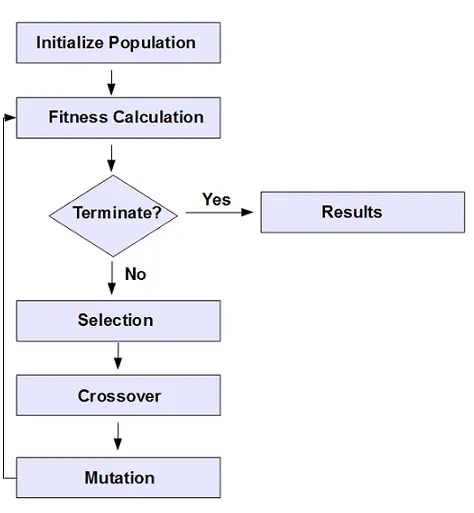
There are steps in genetics algorithm:

1. Initial Population
2. Fitness function
3. Selection
4. Crossover
5. Mutation

Initial Population: The process begins with a set of individuals which is called a Population. Each individual is a solution to the problem you want to solve An individual is characterized by a set of parameters (variables) known as Genes. Genes are joined into a string to form a Chromosome (solution). In a genetic algorithm, the set of genes of an individual is represented using a string, in terms of an alphabet. Usually, binary values are used (string of 1s and 0s). We say that we encode the genes in a chromosome.

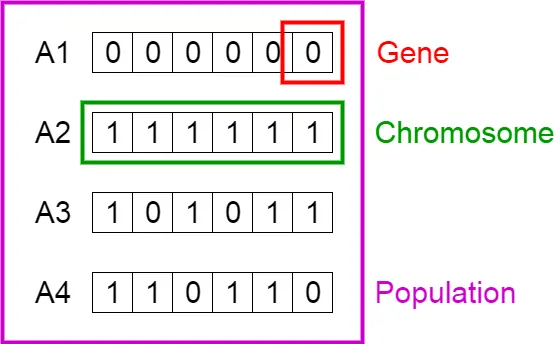
Fitness Function: The fitness function determines how to fit an individual is (the ability of an individual to compete with other individuals). It gives a fitness score to each individual. The probability that an individual will be selected for reproduction is based on its fitness score.

Selection: The idea of selection phase is to select the fittest individuals and let them pass their genes to the next generation.

Two pairs of individuals (parents) are selected based on their fitness scores. Individuals with high fitness have more chance to be selected for reproduction.

Crossover: Crossover is the most significant phase of a genetic algorithm. For each pair of parents to be mated, a crossover point is chosen at random from within the genes.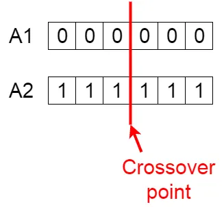

Offspring are created by exchanging the genes of parents among themselves until the crossover point is reached.

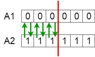
The new offspring are added to the population.

Mutation: In certain new offspring formed, some of their genes can be subjected to a mutation with a low random probability. This implies that some of the bits in the bit string can be flipped.

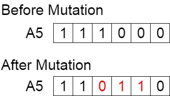
The mutation occurs to maintain diversity within the population and prevent premature convergence.

Termination: The algorithm terminates if the population has converged (does not produce offspring which are significantly different from the previous generation). Then it is said that the genetic algorithm has provided a set of solutions to our problem

flow chart :

• GOVERNING EQUATIONS :

⇒f(x,y)=f1,x⋅f2,x⋅f1,y⋅f2,y">⇒`f(x,y)=f1,x⋅f2,x⋅f1,y⋅f2,y`

⇒f1,x=(sin(5.1πx+0.5))6">⇒`f1,x=(sin(5.1πx+0.5))6`

⇒f1,y=(sin(5.1πy+0.5))6">⇒`f1,y=(sin(5.1πy+0.5))6`

⇒f2,x=exp(-4ln(2)((x-0.0667)20.64))">⇒`f2,x=exp(−4ln(2)((x−0.0667)^2 /(0.64)))` ,

⇒f2,y=exp(-4ln(2)((y-0.0667)20.64))">⇒f`2,y=exp(−4ln(2)((y−0.0667)^2 /0.64)) )`

• Description of syntax of "ga" :

x = ga(fun,nvars) finds a local unconstrained minimum, x, to the objective function, fun. nvars is the dimension (number of design variables) of fun.

function [f] = stalagmite(input_value)

f_1_x = (sin(5.1*pi*input_value(1) + 0.5))^6;
f_1_y = (sin(5.1*pi*input_value(2) + 0.5))^6;
f_2_x = exp(-4*log(2)*(((input_value(1) - 0.0667)^2)/(0.64)));
f_2_y = exp(-4*log(2)*(((input_value(2) - 0.0667)^2)/(0.64)));

f = -(f_1_x*f_1_y*f_2_x*f_2_y);
end

code explanation :

The above function defines the stalagmite function which will be used in the main function.

ii.) The input vectors 'x' and 'y' will be assigned with the required values in the main function.

iii.) Negative sign used in the last line is used to maximize the stalagmite function.

study_1 : unbounded

% A program to calculate the maxima of a function with unbounded inputs

clear all
close all
clc

% inputs for search space

x=linspace(0,0.6,150);
y=linspace(0,0.6,150);

% number of iterations
num_cases=50;

% creating  a 2_dimensional mesh

[xx,yy] = meshgrid(x,y);

% evaluating the stalagmite function

for i = 1:length(xx)
    for j = 1:length(yy)
        input_vector(1) = xx(i,j);
        input_vector(2) = yy(i,j);
        f(i,j) = stalagmite(input_vector);
    end
end

tic
% Study1-Statistical behaviour with unbounded input values

for a=1:num_cases
    [inputs,fopt_1(a)]=ga(@stalagmite,2);
    x_optimum(a)=inputs(1);
    y_optimum(a)=inputs(2);
end
study1_time= toc

% plotting our data

figure(1)
subplot(2,1,1)
hold on
surfc(x,y,-f)
shading interp
colorbar
plot3(x_optimum,y_optimum,-fopt_1,'marker','o','markerfacecolor','r','markersize',5)
title('Unbounded inputs')
subplot(2,1,2)
plot(-fopt_1)
xlabel('Iterations')
ylabel('Function maximum')

matlab code explanation

First two input variables (x and y) were created which were one dimensional arrays of 150 equally spaced values between 0 and 0.6 using linspace command and then two dimensional matrix of these variables were created using meshgrid command. using the meshgrid command, row vectors x and y are converted into matrices xx and yy.we define num_case as 50 which runs 50 itterations With the help of for loop, the input vectors required for stalagmite function are defined using the matrices xx and yy. now we are making use of 2 for loops to mm input for stalagmite function, here we are measuring the time taken for the itteration.by using tic and tok command where tic command is used to start a timer AND toc command is used to stop the timer and the output is stored in study_time 1

Then ga code is entered for unbounded statistical study which have the following format :

[inputs,fopt] = ga(fun,nvars)

Inputs represent the values of parameters x and y for which the function has the least value (fopt)

fun - The function to be optimized, in this case Stalagmite

nvars - the number of design variables, in this case only x and y are the variables to be plotted

now we are plotting the graph from the values we got in itterations from the ga function, here we are making use of the subplot to differerent plots in the same plot, and we are also plotting a 2D plot of optimum function. The surfc command is used to plot contour with xx value and yy value from the mesh grid as input and negative optimum value is used because we need to maximize the function Then shading interp is used to smoothen the function plot and to remove the grid lines Then plot 3 command is used to plot a point in 3 dimensions,here it will plot -fopt because we need the maximum value of the function not the minimum Then x,y axis are labeled .

output plot

Study 1: It can be clearly seen that the values are spread across and the disparity is observed. and unbounded inputs, during each iterations the maximum values changes from 0 to 1,

study_2 : bounded

% A program to calculate the maxima of a function with bounded inputs

clear all
close all
clc

% inputs for search space

x=linspace(0,0.6,150);
y=linspace(0,0.6,150);

% number of iterations
num_cases=50;

% creating  a 2_dimensional mesh

[xx,yy] = meshgrid(x,y);

% evaluating the stalagmite function

for i = 1:length(xx)
    for j = 1:length(yy)
        input_vector(1) = xx(i,j);
        input_vector(2) = yy(i,j);
        f(i,j) = stalagmite(input_vector);
    end
end

tic
% Study2-Statistical behaviour with upper and lower bounded input values

for b=1:num_cases
    [inputs,fopt_2(b)]= ga(@stalagmite,2,[],[],[],[],[0;0],[1;1]);
    x_optimum(b)=inputs(1);
    y_optimum(b)=inputs(2);
end
study2_time = toc

% plotting our data

figure(2)
subplot(2,1,1)
hold on
surfc(x,y,-f)
shading interp
colorbar
plot3(x_optimum,y_optimum,-fopt_2,'marker','o','markerfacecolor','r','markersize',5)
title('Bounded inputs')
subplot(2,1,2)
plot(-fopt_2)
xlabel('Iterations')
ylabel('Function maximum')

code explanation :

similar to the approach as that of study 1, except for the fact that the values are restricted within a range to arrive at a more accurate value as that of the earlier approach.

• the same study is made but this time it is bounded (has lower and upper limit) which requires the same commands and steps except the ga command which have the following format:

[inputs,fopt] = ga(fun,nvars,A,b,Aeq,beq,lb,ub)

Inputs, fopt,fun and nvars are the same as Study 1
A - Linear inequality constraints : real matrix, if there are none, then []
b - Linear inequality constraints : real vector, if there are none, then []
Aeq - Linear equality constraints : real matrix, if there are none, then []
beq - Linear equality constraints : real vector, if there are none, then []
lb - Lower bounds, specified as a real vector or array
ub - Upper bounds, specified as a real vector or array

• here f_opt is the function we are using to storing the optimum function values, x_optimum and y_optimum are the inputs values of the stalagmite for the case study 2.
• we define num_case as 50 which runs 50 itterations, now we are making use of 2 for loops to cenerate input for stalagmite function, here we are measuring the time taken for the itteration as well.
• the ga inbuilt function does the genetic algorithm for us for the defined stalagmite function for different itterations.
• now we are plotting the graph from the values we got in itterations from the ga function, here we are making use of the subplot to differerent plots in the same plot, and we are also plotting a 2D plot of optimum function

output plot

STUDY 2:

Similar to the approach as that of study 1, except for the fact that the values are restricted within a range to arrive at a more accurate value and study of bounded inputs "ga" command is changed and upper and lower bounds of 0 and 1 are set respectively. In this case, the results obtained are much sophisticated as compared to first one.

study_3 : bounded with increse population size

% A program to calculate the maxima of a function with bounded inputs and
% increasing iterations

clear all
close all
clc

% inputs for search space

x=linspace(0,0.6,150);
y=linspace(0,0.6,150);
num_cases=50;

% creating  a 2_dimensional mesh

[xx,yy] = meshgrid(x,y);

% evaluating the stalagmite function

for i = 1:length(xx)
    for j = 1:length(yy)
        input_vector(1) = xx(i,j);
        input_vector(2) = yy(i,j);
        f(i,j) = stalagmite(input_vector);
    end
end

% Study3-Statistical behaviour with upper and lower bounded input values
% and increasing genetic algorithm iterations

option_1 = optimoptions('ga');
option_1 = optimoptions(option_1,'Populationsize',300);

tic
for c=1:num_cases
    [inputs,fopt_3(c)]= ga(@stalagmite,2,[],[],[],[],[0;0],[1;1],[],[],option_1);
    x_optimum(c)=inputs(1);
    y_optimum(c)=inputs(2);
end
study3_time = toc

% plotting our data

figure(3)
subplot(2,1,1)
hold on
surfc(x,y,-f)
shading interp
colorbar
plot3(x_optimum,y_optimum,-fopt_3,'marker','o','markerfacecolor','r','markersize',5)
title('Bounded inputs with increasing population size')
subplot(2,1,2)
plot(-fopt_3)
xlabel('Iterations')
ylabel('Function maximum')

code explnation :

An enhanced study to achieve better results is attained by ensuring and enabling an increase in the initial population size and by using the restricted search space. in the 3rd case study we are incresing the population size ,

• increasing population size study was done which is the same as before but it had different ga code of:

[inputs,fopt]=ga(fun,nvars,A,b,Aeq,beq,lb,ub,nonlcon,IntCon,options)

inputs, fopt,fun and nvars,A,b,Aeq,beq,lb,ub are the same as Study 1 and Study 2 respectively)

nonlcon - Nonlinear constraints, specified as a function handle or function name. If there are none,then []
IntCon - Integer variables, specified as a vector of positive integers, if there are none, then []
Options - Optimization options, specified as the output of optimoptions or a structure.

the range of the genetic algorithm is Bounded as in Study 2 but to improve the accuracy, the commands optimoptions is introduced to increase the Population Size.

negative sign is used to get the maximum value so we can optain the global maxima.

outputs plot :

we are defining the population size as 300 now the itteration would take more time but we would end up with fewer maxima where we can obtain the global maxima,

• conclusion : by using genetic algoritum we can find gobal maxima and gobal minima which intern help to us optimize our error
• refrences : https://en.wikipedia.org/wiki/Genetic_algorithm

https://in.mathworks.com/help/gads/ga.html