Solving second order ODEs

• AIM : To simulate the transient behaviour of a simple pendulum and to create an animation of it's motion on MATLAB
• objective this poject is about the how to calculate the simple harmonic motion in simple pendulum using MATLAB and how to make the animation in this MATLAB code ODE function has been used to solve the problem.
• Theory

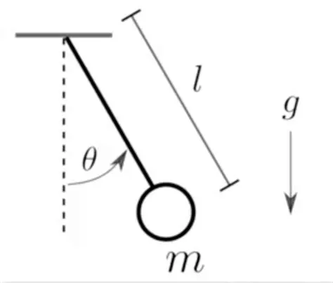
A simple pendulum consist of a metal mass held by a string to a stationary wall.The mass oscillates because of gravity and its inertia when lifted and then left to fall.This oscillation can be modeled using second order differential equation. The way the pendulum moves depends on the Newtons second law. When this law is written down, we get a second order Ordinary Differential Equation that describes the position of the "ball" w.r.t time.

We consider a simple pendulum that consists of a mass m suspended by a string or rod of length L (and negligible mass). The angle it makes with the vertical varies with time as a sine or cosine.

Governing equation

The ODE which represents the equation of motion of simple pendulum with damping is

In the above equation,

g = gravity in m/s2,

L = length of the pendulum in m,

m = mass of the ball in kg,

b=damping coefficient

In mathematics, an ordinary differential equation (ODE) is a differerntial equation containing one or more functions of one independent variable and the derivatives of those functions. The term ordinary is used in contrast with the term partial differential equation which may be with respect to more than one independent variable

The above given codes are for the function to solve the ode,here we are giving the inputs and breaking the 2nd order ode to 2 simple first order odes.

function code

function [dtheta_dt ] = ode_func(t,theta,b,g,l,m)
theta1 = theta(1)
theta2 = theta(2)
dtheta1_dt = theta2;
dtheta2_dt = -(b/m)*theta2 - (g/l)*sin(theta1);
dtheta_dt = [dtheta1_dt;dtheta2_dt];
end

code explanation :

• now create a code for main function first type the inputs to be given - length(l) = 1m, mass(m) = 0.1kg, damping(b) = 0.05, gravity(g) = 9.81 we are giving the intial condition as theta[0, 5] which means that the intial displacement is 0 and initial velocity as 5 rad/sec. next we are using linspace command to generate values 500 values between 0 and 10 second for the time span
• ode45 command is used for solving ode which contains dependent and independent variable along with function, integration limit and inital conditions are provided.
• Function is defined, which is used in ode45 command, to solve the right hand side part of equation at various value of time span.where '@' means call function of the given second order ODE equation with reference to time and initial condition. And "ode_func" is the function definition to represent how the function is defined. Then the graph for the ODE has been plotted with respect to time.
• The results are in the form of two column of which one represent position while the other represent angular velocity vector.
• angular displacement and velocity are plotted from plot command now we are going to create a animation for the pendulum with the values which we obtained from solving the equation.now we create a figure window, and initiate the counter to 1,We open a for loop using a variable i ranging from 1 to length of theta upper end and lower end is fixed so we can initiate x_fixed and y_fixed is 0, and we calculate the end points x_freedom and y_freedom as the end points are moving with respect to the displacement and velocity Then x_freedom and y_freedomI is defined using geometric relation and uses the output angular displacement in column 1 and uses the counter ‘i’ for row counter Then the pendulum string is plotted using array brackets and The the ball of the pendulum is plotted using a marker 0

Then axis is defined and pause command maintains a time interval of 0.01 sec between each pass of i values. then hold off was used to remove the plot in order to have only one plot on the screen after hold on was used to draw all the elements of the plot The multiple figure obtained are saved using getframe command.Using frame captured during looping, movie is created in MATLAB.

main code

clear all
close all
clc
b = 0.05;
g = 9.81;
l = 1;
m = 0.1;
%initialcondition 
theta_0 = [0;5] ;
%times point 
t_span = linspace(0,10,500);
%slove ode
[t,results] = ode45(@(t,theta) ode_func(t,theta,b,g,l,m),t_span,theta_0);
 
plot(t,results(:,1))
hold on
plot(t,results(:,2))
ylabel('displacement&velocity')
xlabel('time')
title('angular velocity v/s time')
legend('displacement','velocity')
%plotting pendulum
figure
ct=1;
for i=1:length(t_span)
x_fixed=0;
y_fixed=0;
x_freeend=l*sin(results(i,1));
y_freeend=-l*cos(results(i,1));
plot([x_fixed x_freeend],[y_fixed y_freeend],[-0.5 0.5],[0 0],'linewidth',3)
hold on
plot(x_freeend,y_freeend,'marker','o','markerSize',30,'markerFacecolor','r')
axis([-1.5 1.5 -1.5 0.5])
grid on
pause(0.01)
M(ct)= getframe(gcf)
ct=ct+1;
hold off
end
movie(M)
videofile=VideoWriter('ode_func.avi','uncompressed AVI');
open(videofile)
writeVideo(videofile,M)
close(videofile)

plot/results :

Plot for Time and AngularVelocity, Displacement

links for the motion of pendulum :

https://youtu.be/ssAHybT9HnE

CONCLUSION:

Thus the program to simulate the transient behaviour of a simple pendulum and to create an animation of it's motion is coded and executed successfully by uploading the video in youtube.