Project 2 - Rankine cycle Simulator

Aim:

The aim of this project is to develop a Rankine Cycle Simulator using MATLAB. The simulator will:

1. Calculate the state points of the Rankine cycle based on user inputs such as turbine inlet temperature, turbine inlet pressure, and condenser inlet pressure.
2. Generate T-s (Temperature-Entropy) and h-s (Enthalpy-Entropy) plots for the calculated state points.
3. Provide essential performance metrics of the Rankine cycle, including net work output and back work ratio.
4. Serve as an educational tool for understanding the thermodynamic principles underlying Rankine cycles and their practical applications in power generation systems.

Objective:

• Calculation of State Points: The simulator will accept user inputs for turbine inlet temperature, turbine inlet pressure, and condenser inlet pressure. Based on these inputs, it will accurately calculate the state points of the Rankine cycle using established thermodynamic relations.

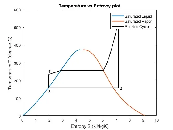
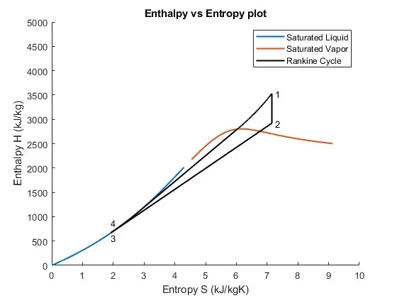
• Generation of T-s and h-s Plots: Upon calculating the state points, the simulator will generate T-s (Temperature-Entropy) and h-s (Enthalpy-Entropy) plots. These plots are crucial for visualizing the thermodynamic processes occurring within the Rankine cycle and aid in understanding its performance.

• Provision of Performance Metrics: The simulator will provide essential performance metrics of the Rankine cycle, including net work output and back work ratio. These metrics are fundamental in evaluating the efficiency and effectiveness of the cycle in power generation applications.

• Educational Tool: The Rankine Cycle Simulator will serve as an educational tool for students and professionals to understand the thermodynamic principles underlying Rankine cycles. By simulating the operation of a Rankine cycle, users can gain insights into its practical applications in power generation systems and deepen their understanding of thermodynamic processes.

Problem Statement:

The problem addressed by this project is the need for a Rankine Cycle Simulator that can accurately calculate the state points of the Rankine cycle and provide visual representations of its thermodynamic processes. The lack of a readily available tool for simulating Rankine cycles hinders the understanding of students and professionals in the field of thermal engineering.

This project aims to develop a MATLAB-based Rankine Cycle Simulator to address this problem. The simulator will take user inputs for turbine inlet temperature, turbine inlet pressure, and condenser inlet pressure, and calculate the corresponding state points of the Rankine cycle. It will generate T-s (Temperature-Entropy) and h-s (Enthalpy-Entropy) plots to visualize the thermodynamic processes and provide essential performance metrics such as net work output and back work ratio.

By developing this Rankine Cycle Simulator, the project seeks to provide a comprehensive educational tool for understanding Rankine cycles and their practical applications in power generation systems.

Rankine Cycle:

The Rankine Cycle is a thermodynamic cycle that is commonly utilized in steam power plants for electricity generation. It represents the idealized process of converting heat energy into mechanical work, which can then be used to drive a turbine and ultimately produce electricity. Here is a theoretical overview of the Rankine Cycle:

1. Boiler (Heat Addition):

   • The cycle begins with the boiler, where water is heated to its boiling point by means of a heat source such as burning coal, natural gas, or nuclear fission.
   • The high-pressure steam generated in the boiler is then expanded through a turbine, where it performs mechanical work by driving the turbine blades.

2. Turbine (Expansion):

   • The high-pressure steam from the boiler enters the turbine, where it expands and loses pressure while simultaneously performing work on the turbine blades.
   • As the steam expands, its temperature and pressure decrease, and its internal energy is converted into mechanical work.

3. Condenser (Heat Rejection):

   • After exiting the turbine, the low-pressure steam is directed to the condenser, where it is condensed back into liquid form by transferring heat to a cooling medium, typically water from a nearby river or cooling tower.
   • The condensation process releases latent heat, which is rejected to the cooling medium, resulting in a significant decrease in pressure and temperature.

4. Pump (Compression):

   • The condensed liquid (now referred to as feedwater) is then pumped back to the boiler at high pressure by a feedwater pump.
   • The feedwater is pressurized to the boiler pressure to complete the cycle.

5. Cycle Completion:

   • The cycle is completed as the high-pressure feedwater enters the boiler, where it is once again heated to its boiling point, thus restarting the process.

Key Concepts:

• Thermal Efficiency: The efficiency of the Rankine Cycle is determined by the ratio of the net work output to the heat input. Higher efficiencies are achieved by maximizing the temperature and pressure differentials within the cycle.

• Back Work Ratio: The back work ratio represents the portion of work output that is required to operate the feedwater pump. It is calculated as the ratio of the work input to the pump to the net work output of the turbine.

• Quality of Steam: The quality of steam refers to the steam's dryness fraction, which indicates the proportion of vapor to liquid in the steam mixture. High-quality steam (closer to 1) is desirable for maximizing turbine efficiency and avoiding erosion of turbine blades.

• Subcooling and Superheating: Subcooling refers to the process of cooling the liquid below its saturation temperature, while superheating involves heating the steam above its saturation temperature. Both processes enhance the efficiency and performance of the Rankine Cycle.

Overall, the Rankine Cycle is a fundamental concept in thermal engineering, providing a theoretical framework for understanding the operation of steam power plants and other heat-driven processes.

Turbine (Process: 1-2) Isentropic Expansion: The process involves isentropic expansion, where the superheated vapor is expanded isentropically in the turbine, producing work that can be converted into electricity. The turbine's exit condition may occur in three states: superheated, saturated vapor, or liquid-vapor mixture.

`W _t = (h1 - h2)`

Condenser (Process: 2-3) Isobaric Heat Rejection: During this process, isobaric heat rejection occurs. The vapor-liquid mixture leaving the turbine is condensed at a constant low pressure, typically in a surface condenser using cooling water. In well-designed and maintained condensers, the vapor pressure is well below atmospheric pressure, approaching the saturation pressure of the operating fluid at the cooling water temperature.

`Q_(out) ​= (h2 - h3)`

Pump (Process: 3-4) Isentropic Compression: This process involves isentropic compression. The pressure of the condensate is raised isentropically in the feed pump. Due to the low specific volume of liquids, the pump work is relatively small and is often neglected in thermodynamic calculations.

`W_p = (h4 - h3)`

Boiler (Process: 4-1) Isobaric Heat Transfer: During isobaric heat transfer, high-pressure liquid enters the boiler from the feed pump and is heated to the saturation temperature. Further addition of energy causes evaporation of the liquid until it is fully converted to saturated steam. Additional energy input takes the saturated steam into a superheated state.

`Q_(i n) = (h1 - h4)`

Other Formula's:

Thermal Efficiency (η):

`eta = W_(n et)/Q_(i n)`

Net Work Output (W_net):

`W_(n et) = W_(t) - W_(p)`

Work Output of Turbine (W_t):

`W _t = (h1 - h2)`

Work Output of Pump (W_p):

`W_p = (h4 - h3)`

Back Work Ratio (BWR):

`BWR = W_p/W_t`

Specific Steam Consumption (SSC):

`SSC = 3600/(W_(n et))`

Input Parameters:

Case 1: Turbine Outlet is either Saturated state or Liquid-vapor mix state:

Pressure at Turbine Inlet (P1) = 30 bar

Temperature at Turbine Inlet (T1) = 400 deg Celcius

Pressure at Condenser Inlet (P2) = 0.05 bar

Case 2: Turbine Outlet is in Superheated state:

Pressure at Turbine Inlet (P1) = 44 bar

Temperature at Turbine Inlet (T1)= 538 deg Celcius

Pressure at Condenser Inlet (P2) = 5.83 bar

Matlab Program:

% Rankine Cycle Simulator
% Objective: Simulate the Rankine cycle and plot T-s and h-s diagrams using XSteam data
% Water and steam properties according to IAPWS IF-97

clear all          % Clear all variables from workspace
close all          % Close all open figures
clc                % Clear command window

%% Input Prompt Section
disp('RANKINE CYCLE SIMULATOR'); % Displaying a title
fprintf('\n');
disp('1-2 is Isentropic Expansion in the Turbine');
disp('2-3 is Constant Pressure Heat Rejection by the Condenser');
disp('3-4 is Isentropic Compression in the Pump');
disp('4-1 is Constant Pressure Heat Addition by the Boiler');

%% Obtaining the input data
p1 = input('\nEnter the Pressure at turbine inlet, p1(in bar) = ');
T1 = input('Enter the Temperature at turbine inlet, T1(in degree.C) = ');
p2 = input('Enter the Pressure at condenser inlet, p2(in bar) = ');

%% Extracting data and defining variables for each state of the cycle

% State 1: Turbine Inlet
h1 = XSteam('h_pT', p1, T1); % Enthalpy at state point 1
s1 = XSteam('s_pT', p1, T1); % Specific entropy at state point 1

% State 2: Turbine Outlet
s2 = s1; % Isentropic expansion, entropy remains constant
sf2= XSteam('sL_p', p2); % Saturated liquid entropy at pressure p2
sg2 = XSteam('sV_p', p2); % Saturated vapor entropy at pressure p2
x2 = (s2-sf2)/(sg2-sf2); % Dryness fraction calculation
hf2 = XSteam('hL_p', p2); % Saturated liquid enthalpy at pressure p2
hg2 = XSteam('hV_p', p2); % Saturated vapor enthalpy at pressure p2
h2 = hf2 + (x2*(hg2-hf2)); % Enthalpy at state point 2

% State 3: Condenser Outlet
p3 = p2; % Pressure remains constant in the condenser
s3 = XSteam('sL_p', p3); % Saturated liquid entropy at pressure p3
h3 = XSteam('hL_p', p3); % Saturated liquid enthalpy at pressure p3

% State 4: Pump Inlet
s4 = s3; % Isentropic compression in the pump, entropy remains constant
p4 = p1; % Pressure remains constant in the boiler

%% Calculate work and heat interactions

% Turbine work
Wt = h1 - h2; % Calculate the work done by the turbine

% Pump work
v3 = XSteam('vL_p', p3); % Saturated liquid specific volume at pressure p3
Wp = v3*(p4 - p3)*100; % Calculate the work done by the pump
h4 = h3 + Wp; % Calculate the enthalpy at state point 4

% Net work
Wnet = Wt - Wp; % Calculate the net work output of the cycle

% Back work ratio
Back_Work_Ratio = Wp/Wt; % Calculate the back work ratio, ratio of pump work to turbine work

% Heat into the system
Qin = h1 - h4; % Calculate the heat added to the system

% Heat out of the system
Qout = h2 - h3; % Calculate the heat rejected by the system

% Thermal efficiency
eff = (Wnet/Qin)*100; % Calculate the thermal efficiency of the cycle

% Specific Steam Consumption
SSC = (3600/Wnet); % Calculate the specific steam consumption, mass flow rate/power

%% Calculate temperatures at state points for plotting

T3 = XSteam('Tsat_p', p3); % Saturation temperature at state point 3
T2 = T3; % Set temperature at state point 2 equal to the saturation temperature at state point 3
Cp4 = XSteam('Cp_ps', p4, s4); % Specific isobaric heat capacity at state point 4
Cv4 = XSteam('Cv_ps', p4, s4); % Specific isochoric heat capacity at state point 4
k = Cp4/Cv4; % Specific heat ratio
T4 = T3/((p3/p4)^((k-1)/k)); % Temperature at state point 4 derived from isentropic relation

% Temperatures and enthalpies at the vapor and liquid lines for plotting
T6 = XSteam('Tsat_p', p1); % Saturation temperature at state point 6 (boiler)
s5 = XSteam('sL_p', p1); % Saturated liquid entropy at pressure p1
s6 = XSteam('sV_p', p1); % Saturated vapor entropy at pressure p1
h5 = XSteam('hL_p', p1); % Saturated liquid enthalpy at pressure p1
h6 = XSteam('hV_p', p1); % Saturated vapor enthalpy at pressure p1
T5 = T6; % Set temperature at state point 5 equal to the saturation temperature at state point 6 (boiler)

%% Plotting the saturation curve

T = linspace(1,400,1000); % Generate an array of temperatures from 1°C to 400°C

% Initialize arrays to store saturated liquid and vapor properties
sf = zeros(size(T)); % Array to store saturated liquid entropy
sg = zeros(size(T)); % Array to store saturated vapor entropy
hf = zeros(size(T)); % Array to store saturated liquid enthalpy
hg = zeros(size(T)); % Array to store saturated vapor enthalpy

% Loop over each temperature point to calculate corresponding properties
for i = 1:length(T)
    sf(i) = XSteam('sL_T', T(i)); % Calculate saturated liquid entropy at temperature T(i)
    sg(i) = XSteam('sV_T', T(i)); % Calculate saturated vapor entropy at temperature T(i)
    hf(i) = XSteam('hL_T', T(i)); % Calculate saturated liquid enthalpy at temperature T(i)
    hg(i) = XSteam('hV_T', T(i)); % Calculate saturated vapor enthalpy at temperature T(i)
end

%% Plotting T-s diagram

figure(1); % Create a new figure for the T-s diagram

% Plotting the saturation lines
plot(sf, T,'linewidth',1.5) % Plot the saturated liquid line
hold on
plot(sg, T,'linewidth',1.5) % Plot the saturated vapor line

% Plotting the processes of the Rankine cycle
plot([s1 s2], [T1 T2], 'k', 'linewidth', 1.5) % Process 1-2 (Isentropic expansion in turbine)
plot([s2 s3], [T2 T3], 'k', 'linewidth', 1.5) % Process 2-3 (Constant pressure heat rejection in condenser)
plot([s3 s4], [T3 T4], 'k', 'linewidth', 1.5) % Process 3-4 (Isentropic compression in pump)
plot([s4 s5], [T4 T5], 'k', 'linewidth', 1.5) % Process 4-1 (Constant pressure heat addition in boiler)
plot([s5 s6], [T5 T6], 'k', 'linewidth', 1.5) % Vapor line

% Plotting the constant pressure line for the boiler
sc1 = linspace(s6, s1, 1000); % Generate entropy values for the constant pressure line
for l = 1:length(sc1)
    Tc1(l) = XSteam('T_ps', p1, sc1(l)); % Calculate temperature as a function of pressure and entropy
end
plot(sc1, Tc1, 'k', 'linewidth', 1.5) % Plot the constant pressure line for the boiler

% Adding text annotations for state points
text(s1+0.1, T1, '1') % Label state point 1
text(s2+0.1, T2, '2') % Label state point 2
text(s3, T3-20, '3') % Label state point 3
text(s4, T4+20, '4') % Label state point 4

% Adding plot titles, axis labels, and legend
title('Temperature vs Entropy plot')
xlabel('Entropy S (kJ/kgK)')
ylabel('Temperature T (degree C) ')
axis([0 10 0 600]) % Set axis limits
legend('Saturated Liquid','Saturated Vapor','Rankine Cycle') % Add legend

%% Plotting h-s diagram

figure(2); % Create a new figure for the h-s diagram

hold on

% Plotting the saturation lines
plot(sf, hf, 'linewidth', 1.5) % Plot the saturated liquid line
plot(sg, hg, 'linewidth', 1.5) % Plot the saturated vapor line

% Plotting the processes of the Rankine cycle
plot([s1 s2], [h1 h2], 'k', 'linewidth', 1.5) % Process 1-2 (Isentropic expansion in turbine)
plot([s2 s3], [h2 h3], 'k', 'linewidth', 1.5) % Process 2-3 (Constant pressure heat rejection in condenser)
plot([s3 s4], [h3 h4], 'k', 'linewidth', 1.5) % Process 3-4 (Isentropic compression in pump)

% Define a vector of enthalpy values between h4 and h5
hc = linspace(h4, h5, 100);

% Calculate specific entropy values corresponding to each enthalpy value
for k = 1:length(hc)
    sch(k) = XSteam('s_ph', p1, hc(k)); % Specific entropy as a function of pressure and enthalpy
end

% Plot the constant pressure line (boiler) on the entropy-enthalpy diagram
plot(sch, hc, 'k', 'linewidth', 1.5) % Constant pressure line (boiler)

% Calculate enthalpy values corresponding to each entropy value in sc1
for m = 1:length(sc1)
    hc1(m) = XSteam('h_ps', p1, sc1(m)); % Enthalpy as a function of pressure and entropy
end

% Plot another constant pressure line (boiler)
plot(sc1, hc1, 'k', 'linewidth', 1.5) % Constant pressure line (boiler)

% Plot the vapor line
plot([s5 s6], [h5 h6], 'k', 'linewidth', 1.5) % Vapor line

% Adding text annotations for state points
text(s1+0.1, h1, '1') % Label state point 1
text(s2+0.1, h2, '2') % Label state point 2
text(s3, h3-100, '3') % Label state point 3
text(s4, h4 +200, '4') % Label state point 4

% Adding plot titles, axis labels, and legend
title('Enthalpy vs Entropy plot')
xlabel('Entropy S (kJ/kgK)')
ylabel('Enthalpy H (kJ/kg)')
axis([0 10 0 5000]) % Set axis limits
legend('Saturated Liquid', 'Saturated Vapor', 'Rankine Cycle') % Add legend

%% Displaying Results

fprintf('\nRESULTS'); % Display a header for the results section

% Display results for state point 1
fprintf('\n\n At State Point 1:');
fprintf('\n p1: %8.3f bar', p1); % Display pressure at state point 1
fprintf('\n T1: %8.3f deg C', T1); % Display temperature at state point 1
fprintf('\n h1: %8.3f KJ/kg', h1); % Display enthalpy at state point 1
fprintf('\n s1: %8.3f KJ/kgK', s1); % Display specific entropy at state point 1

% Display results for state point 2
fprintf('\n\n At State Point 2:');
fprintf('\n p2: %8.3f bar', p2); % Display pressure at state point 2
fprintf('\n T2: %8.3f deg C', T2); % Display temperature at state point 2
fprintf('\n h2: %8.3f kJ/kg', h2); % Display enthalpy at state point 2
fprintf('\n s2: %8.3f kJ/kgK', s2); % Display specific entropy at state point 2
fprintf('\n x2: %8.3f', x2); % Display dryness fraction at state point 2

% Display results for state point 3
fprintf('\n\n At State Point 3:');
fprintf('\n p3: %8.3f bar', p3); % Display pressure at state point 3
fprintf('\n T3: %8.3f deg C', T3); % Display temperature at state point 3
fprintf('\n h3: %8.3f kJ/kg', h3); % Display enthalpy at state point 3
fprintf('\n s3: %8.3f kJ/kgK', s3); % Display specific entropy at state point 3

% Display results for state point 4
fprintf('\n\n At State Point 4:');
fprintf('\n p4: %8.3f bar', p4); % Display pressure at state point 4
fprintf('\n T4: %8.3f deg C', T4); % Display temperature at state point 4
fprintf('\n h4: %8.3f kJ/kg', h4); % Display enthalpy at state point 4
fprintf('\n s4: %8.3f kJ/kgK', s4); % Display specific entropy at state point 4

% Display turbine work
fprintf('\n\n Turbine Work: %.3f kJ/kg', Wt); % Display turbine work

% Display pump work
fprintf('\n Pump Work: %.3f kJ/kg', Wp); % Display pump work

% Display net work
fprintf('\n Net Work Output: %.3f kJ/kg', Wnet); % Display net work

% Display back work ratio
fprintf('\n Back Work Ratio: %.3f ',Back_Work_Ratio); % Display back work ratio

% Display thermal efficiency
fprintf('\n Efficiency: %.3f Percent ', eff); % Display thermal efficiency

% Display specific steam consumption
fprintf('\n S.S.C: %.3f kJ/kWh\n', SSC); % Display specific steam consumption

Explanation:

Clear Workspace and Command Window

clear all          % Clear all variables from workspace
close all          % Close all open figures
clc                % Clear command window

This section ensures a clean workspace by clearing all variables, closing all figures, and clearing the command window.

Input Prompt Section

disp('RANKINE CYCLE SIMULATOR'); % Displaying a title
fprintf('\n');
disp('1-2 is Isentropic Expansion in the Turbine');
disp('2-3 is Constant Pressure Heat Rejection by the Condenser');
disp('3-4 is Isentropic Compression in the Pump');
disp('4-1 is Constant Pressure Heat Addition by the Boiler');

Here, a title and explanations about the different processes in the Rankine cycle are displayed.

Obtaining the Input Data

p1 = input('\nEnter the Pressure at turbine inlet, p1(in bar) = ');
T1 = input('Enter the Temperature at turbine inlet, T1(in degree.C) = ');
p2 = input('Enter the Pressure at condenser inlet, p2(in bar) = ');

This section prompts the user to input data such as pressure and temperature values.

Extracting Data and Defining Variables for Each State of the Cycle

% State 1: Turbine Inlet
h1 = XSteam('h_pT', p1, T1); % Enthalpy at state point 1
s1 = XSteam('s_pT', p1, T1); % Specific entropy at state point 1

% State 2: Turbine Outlet
s2 = s1; % Isentropic expansion, entropy remains constant
sf2= XSteam('sL_p', p2); % Saturated liquid entropy at pressure p2
sg2 = XSteam('sV_p', p2); % Saturated vapor entropy at pressure p2
x2 = (s2-sf2)/(sg2-sf2); % Dryness fraction calculation
hf2 = XSteam('hL_p', p2); % Saturated liquid enthalpy at pressure p2
hg2 = XSteam('hV_p', p2); % Saturated vapor enthalpy at pressure p2
h2 = hf2 + (x2*(hg2-hf2)); % Enthalpy at state point 2

% State 3: Condenser Outlet
p3 = p2; % Pressure remains constant in the condenser
s3 = XSteam('sL_p', p3); % Saturated liquid entropy at pressure p3
h3 = XSteam('hL_p', p3); % Saturated liquid enthalpy at pressure p3

% State 4: Pump Inlet
s4 = s3; % Isentropic compression in the pump, entropy remains constant
p4 = p1; % Pressure remains constant in the boiler

This section calculates properties for each state of the cycle using XSteam functions based on pressure and temperature inputs.

1. State 1: Turbine Inlet

   • h1 = XSteam('h_pT', p1, T1);: This line calculates the enthalpy (h1) at state point 1 using the pressure (p1) and temperature (T1) provided. It seems to be using a function XSteam to obtain thermodynamic properties from steam tables or equations of state.

   • s1 = XSteam('s_pT', p1, T1);: Similarly, this line calculates the specific entropy (s1) at state point 1 using the same function XSteam.

2. State 2: Turbine Outlet

   • s2 = s1;: This line assumes isentropic expansion, meaning the entropy remains constant during the expansion process.

   • sf2= XSteam('sL_p', p2); and sg2 = XSteam('sV_p', p2);: These lines calculate the entropy of saturated liquid (sf2) and saturated vapor (sg2) at the pressure (p2) provided.

   • x2 = (s2-sf2)/(sg2-sf2);: This line calculates the dryness fraction (x2) of the steam at state point 2 using the difference between the actual entropy (s2) and the entropy of saturated liquid (sf2), normalized by the difference between the entropy of saturated vapor (sg2) and the entropy of saturated liquid (sf2).

   • hf2 = XSteam('hL_p', p2); and hg2 = XSteam('hV_p', p2);: These lines calculate the enthalpy of saturated liquid (hf2) and saturated vapor (hg2) at the pressure (p2) provided.

   • h2 = hf2 + (x2*(hg2-hf2));: This line calculates the enthalpy (h2) at state point 2 using the dryness fraction (x2) calculated earlier.

3. State 3: Condenser Outlet

   • p3 = p2;: This line sets the pressure at state point 3 to be equal to the pressure at state point 2 since pressure typically remains constant in the condenser.

   • s3 = XSteam('sL_p', p3);: This line calculates the entropy of saturated liquid (s3) at the pressure (p3) provided.

   • h3 = XSteam('hL_p', p3);: This line calculates the enthalpy of saturated liquid (h3) at the pressure (p3) provided.

4. State 4: Pump Inlet

   • s4 = s3;: This line assumes isentropic compression, meaning the entropy remains constant during the compression process.

   • p4 = p1;: This line sets the pressure at state point 4 to be equal to the pressure at state point 1 since pressure typically remains constant in the boiler.

Calculating Temperatures at State Points for Plotting

T3 = XSteam('Tsat_p', p3); % Saturation temperature at state point 3
T2 = T3; % Set temperature at state point 2 equal to the saturation temperature at state point 3
Cp4 = XSteam('Cp_ps', p4, s4); % Specific isobaric heat capacity at state point 4
Cv4 = XSteam('Cv_ps', p4, s4); % Specific isochoric heat capacity at state point 4
k = Cp4/Cv4; % Specific heat ratio
T4 = T3/((p3/p4)^((k-1)/k)); % Temperature at state point 4 derived from isentropic relation

This section calculates temperatures at different state points using XSteam functions and thermodynamic relations.

1. State 3: Condenser Outlet

   • T3 = XSteam('Tsat_p', p3);: This line calculates the saturation temperature (T3) at state point 3 using the pressure (p3) provided. The function XSteam is used to obtain this information from steam tables or equations of state.

2. State 2: Turbine Outlet

   • T2 = T3;: This line sets the temperature at state point 2 to be equal to the saturation temperature at state point 3 (T3). This is typically a reasonable approximation for isentropic expansion in a steam turbine.

3. State 4: Pump Inlet

   • Cp4 = XSteam('Cp_ps', p4, s4);: This line calculates the specific isobaric heat capacity (Cp4) at state point 4 using the pressure (p4) and specific entropy (s4) provided. Isobaric heat capacity represents the amount of heat required to raise the temperature of a substance at constant pressure.

   • Cv4 = XSteam('Cv_ps', p4, s4);: Similarly, this line calculates the specific isochoric heat capacity (Cv4) at state point 4 using the same pressure (p4) and specific entropy (s4). Isochoric heat capacity represents the amount of heat required to raise the temperature of a substance at constant volume.

   • k = Cp4/Cv4;: This line calculates the specific heat ratio (k) using the ratio of specific isobaric heat capacity (Cp4) to specific isochoric heat capacity (Cv4). The specific heat ratio is an important parameter in thermodynamics, particularly in the context of ideal gases.

   • T4 = T3/((p3/p4)^((k-1)/k));: This line calculates the temperature (T4) at state point 4 using the isentropic relation derived from the specific heat ratio (k). The isentropic relation describes the relationship between temperature, pressure, and specific heat ratio during an isentropic process, such as the compression of a fluid in a pump.

Plotting the Saturation Curve

T = linspace(1,400,1000); % Generate an array of temperatures from 1°C to 400°C

% Initialize arrays to store saturated liquid and vapor properties
sf = zeros(size(T)); % Array to store saturated liquid entropy
sg = zeros(size(T)); % Array to store saturated vapor entropy
hf = zeros(size(T)); % Array to store saturated liquid enthalpy
hg = zeros(size(T)); % Array to store saturated vapor enthalpy

% Loop over each temperature point to calculate corresponding properties
for i = 1:length(T)
    sf(i) = XSteam('sL_T', T(i)); % Calculate saturated liquid entropy at temperature T(i)
    sg(i) = XSteam('sV_T', T(i)); % Calculate saturated vapor entropy at temperature T(i)
    hf(i) = XSteam('hL_T', T(i)); % Calculate saturated liquid enthalpy at temperature T(i)
    hg(i) = XSteam('hV_T', T(i)); % Calculate saturated vapor enthalpy at temperature T(i)
end

This section generates data for the saturation curve by calculating saturated liquid and vapor properties over a range of temperatures using XSteam functions.

1. Generating Array of Temperatures

   • T = linspace(1,400,1000);: This line generates an array of 1000 temperature points (T) ranging from 1°C to 400°C using the linspace function. This array will be used to calculate thermodynamic properties at various temperatures.

2. Initializing Arrays

   • sf = zeros(size(T));, sg = zeros(size(T));, hf = zeros(size(T));, hg = zeros(size(T));: These lines initialize arrays (sf, sg, hf, hg) with the same size as the temperature array T. These arrays will store the calculated values of saturated liquid entropy (sf), saturated vapor entropy (sg), saturated liquid enthalpy (hf), and saturated vapor enthalpy (hg) corresponding to each temperature point.

3. Looping Over Temperature Points

   • for i = 1:length(T): This line starts a loop that iterates over each temperature point in the array T.

   • sf(i) = XSteam('sL_T', T(i));: Inside the loop, this line calculates the saturated liquid entropy (sf(i)) at the temperature T(i) using the function XSteam, which likely retrieves this information from steam tables or equations of state.

   • sg(i) = XSteam('sV_T', T(i));: Similarly, this line calculates the saturated vapor entropy (sg(i)) at the temperature T(i).

   • hf(i) = XSteam('hL_T', T(i));: This line calculates the saturated liquid enthalpy (hf(i)) at the temperature T(i).

   • hg(i) = XSteam('hV_T', T(i));: This line calculates the saturated vapor enthalpy (hg(i)) at the temperature T(i).

4. Explanation of Calculations

   • XSteam is a function likely used to obtain thermodynamic properties of water and steam. The inputs to this function ('sL_T', 'sV_T', 'hL_T', 'hV_T') specify the property being requested (saturated liquid/vapor entropy or enthalpy) at a given temperature.
   • The loop iterates over each temperature point, and for each point, it calculates the corresponding values of saturated liquid and vapor properties using the XSteam function.
   • The calculated values are stored in the respective arrays (sf, sg, hf, hg) for further analysis or plotting.

Plotting T-s Diagram

figure(1); % Create a new figure for the T-s diagram

% Plotting the saturation lines
plot(sf, T,'linewidth',1.5) % Plot the saturated liquid line
hold on
plot(sg, T,'linewidth',1.5) % Plot the saturated vapor line

% Plotting the processes of the Rankine cycle
plot([s1 s2], [T1 T2], 'k', 'linewidth', 1.5) % Process 1-2 (Isentropic expansion in turbine)
plot([s2 s3], [T2 T3], 'k', 'linewidth', 1.5) % Process 2-3 (Constant pressure heat rejection in condenser)
plot([s3 s4], [T3 T4], 'k', 'linewidth', 1.5) % Process 3-4 (Isentropic compression in pump)
plot([s4 s5], [T4 T5], 'k', 'linewidth', 1.5) % Process 4-1 (Constant pressure heat addition in boiler)
plot([s5 s6], [T5 T6], 'k', 'linewidth', 1.5) % Vapor line

% Plotting the constant pressure line for the boiler
sc1 = linspace(s6, s1, 1000); % Generate entropy values for the constant pressure line
for l = 1:length(sc1)
    Tc1(l) = XSteam('T_ps', p1, sc1(l)); % Calculate temperature as a function of pressure and entropy
end
plot(sc1, Tc1, 'k', 'linewidth', 1.5) % Plot the constant pressure line for the boiler

% Adding text annotations for state points
text(s1+0.1, T1, '1') % Label state point 1
text(s2+0.1, T2, '2') % Label state point 2
text(s3, T3-20, '3') % Label state point 3
text(s4, T4+20, '4') % Label state point 4

% Adding plot titles, axis labels, and legend
title('Temperature vs Entropy plot')
xlabel('Entropy S (kJ/kgK)')
ylabel('Temperature T (degree C) ')
axis([0 10 0 600]) % Set axis limits
legend('Saturated Liquid','Saturated Vapor','Rankine Cycle') % Add legend

This section creates a new figure for the T-s (Temperature-Entropy) diagram. It plots the saturated liquid and vapor lines, along with the processes of the Rankine cycle. Annotations and labels are added to the plot, and a legend is included.

1. Creating a New Figure

   • figure(1);: This line creates a new figure window for the T-s diagram.

2. Plotting Saturation Lines

   • plot(sf, T,'linewidth',1.5): This line plots the saturated liquid line on the T-s diagram, where sf is the array of saturated liquid entropy values and T is the corresponding temperature array.

   • plot(sg, T,'linewidth',1.5): Similarly, this line plots the saturated vapor line on the T-s diagram, using the array sg for saturated vapor entropy.

3. Plotting Processes of the Rankine Cycle

   • plot([s1 s2], [T1 T2], 'k', 'linewidth', 1.5): This line plots Process 1-2, which represents the isentropic expansion in the turbine, connecting state points 1 and 2 on the diagram.

   • plot([s2 s3], [T2 T3], 'k', 'linewidth', 1.5): This line plots Process 2-3, representing the constant pressure heat rejection in the condenser.

   • plot([s3 s4], [T3 T4], 'k', 'linewidth', 1.5): This line plots Process 3-4, representing the isentropic compression in the pump.

   • plot([s4 s5], [T4 T5], 'k', 'linewidth', 1.5): This line plots Process 4-1, representing the constant pressure heat addition in the boiler.

   • plot([s5 s6], [T5 T6], 'k', 'linewidth', 1.5): This line plots the vapor line.

4. Plotting Constant Pressure Line for the Boiler

   • sc1 = linspace(s6, s1, 1000);: This line generates entropy values (sc1) for the constant pressure line in the boiler by creating a linear space between the entropy values at state points 6 and 1.

   • for l = 1:length(sc1) ... end: This loop calculates the corresponding temperature (Tc1) for each entropy value sc1 using the function XSteam.

   • plot(sc1, Tc1, 'k', 'linewidth', 1.5): This line plots the constant pressure line for the boiler on the T-s diagram.

5. Adding Annotations

   • text(s1+0.1, T1, '1'): This line adds a text annotation '1' near state point 1 on the diagram.

   • text(s2+0.1, T2, '2'): Similarly, this line adds a text annotation '2' near state point 2.

   • text(s3, T3-20, '3'): This line adds a text annotation '3' near state point 3.

   • text(s4, T4+20, '4'): This line adds a text annotation '4' near state point 4.

6. Titles, Labels, and Legend

   • title('Temperature vs Entropy plot'): This line sets the title of the T-s diagram.

   • xlabel('Entropy S (kJ/kgK)'): This line labels the x-axis as 'Entropy'.

   • ylabel('Temperature T (degree C) '): This line labels the y-axis as 'Temperature'.

   • axis([0 10 0 600]): This line sets the limits for the x-axis and y-axis.

   • legend('Saturated Liquid','Saturated Vapor','Rankine Cycle'): This line adds a legend to the diagram, indicating the plotted lines.

Plotting h-s Diagram

figure(2); % Create a new figure for the h-s diagram

hold on

% Plotting the saturation lines
plot(sf, hf, 'linewidth', 1.5) % Plot the saturated liquid line
plot(sg, hg, 'linewidth', 1.5) % Plot the saturated vapor line

% Plotting the processes of the Rankine cycle
plot([s1 s2], [h1 h2], 'k', 'linewidth', 1.5) % Process 1-2 (Isentropic expansion in turbine)
plot([s2 s3], [h2 h3], 'k', 'linewidth', 1.5) % Process 2-3 (Constant pressure heat rejection in condenser)
plot([s3 s4], [h3 h4], 'k', 'linewidth', 1.5) % Process 3-4 (Isentropic compression in pump)

% Define a vector of enthalpy values between h4 and h5
hc = linspace(h4, h5, 100);

% Calculate specific entropy values corresponding to each enthalpy value
for k = 1:length(hc)
    sch(k) = XSteam('s_ph', p1, hc(k)); % Specific entropy as a function of pressure and enthalpy
end

% Plot the constant pressure line (boiler) on the entropy-enthalpy diagram
plot(sch, hc, 'k', 'linewidth', 1.5) % Constant pressure line (boiler)

% Calculate enthalpy values corresponding to each entropy value in sc1
for m = 1:length(sc1)
    hc1(m) = XSteam('h_ps', p1, sc1(m)); % Enthalpy as a function of pressure and entropy
end

% Plot another constant pressure line (boiler)
plot(sc1, hc1, 'k', 'linewidth', 1.5) % Constant pressure line (boiler)

% Plot the vapor line
plot([s5 s6], [h5 h6], 'k', 'linewidth', 1.5) % Vapor line

% Adding text annotations for state points
text(s1+0.1, h1, '1') % Label state point 1
text(s2+0.1, h2, '2') % Label state point 2
text(s3, h3-100, '3') % Label state point 3
text(s4, h4 +200, '4') % Label state point 4

% Adding plot titles, axis labels, and legend
title('Enthalpy vs Entropy plot')
xlabel('Entropy S (kJ/kgK)')
ylabel('Enthalpy H (kJ/kg)')
axis([0 10 0 5000]) % Set axis limits
legend('Saturated Liquid', 'Saturated Vapor', 'Rankine Cycle') % Add legend

This section creates a new figure for the h-s (Enthalpy-Entropy) diagram. It plots the saturated liquid and vapor lines, along with the processes of the Rankine cycle. Annotations and labels are added to the plot, and a legend is included.

1. Creating a New Figure

   • figure(2);: This line creates a new figure window for the h-s diagram.

2. Plotting Saturation Lines

   • plot(sf, hf, 'linewidth', 1.5): This line plots the saturated liquid line on the h-s diagram, where sf is the array of saturated liquid entropy values and hf is the corresponding array of saturated liquid enthalpy values.

   • plot(sg, hg, 'linewidth', 1.5): Similarly, this line plots the saturated vapor line on the h-s diagram, using the arrays sg and hg for saturated vapor entropy and enthalpy, respectively.

3. Plotting Processes of the Rankine Cycle

   • plot([s1 s2], [h1 h2], 'k', 'linewidth', 1.5): This line plots Process 1-2, representing the isentropic expansion in the turbine, connecting state points 1 and 2 on the diagram.

   • plot([s2 s3], [h2 h3], 'k', 'linewidth', 1.5): This line plots Process 2-3, representing the constant pressure heat rejection in the condenser.

   • plot([s3 s4], [h3 h4], 'k', 'linewidth', 1.5): This line plots Process 3-4, representing the isentropic compression in the pump.

4. Constant Pressure Lines for the Boiler

   • hc = linspace(h4, h5, 100);: This line generates a vector of enthalpy values (hc) between h4 and h5 to plot the constant pressure line (boiler) on the h-s diagram.

   • for k = 1:length(hc) ... end: This loop calculates the corresponding specific entropy values (sch) for each enthalpy value in hc using the function XSteam.

   • plot(sch, hc, 'k', 'linewidth', 1.5): This line plots the constant pressure line (boiler) on the h-s diagram.

5. Plotting the Vapor Line

   • plot([s5 s6], [h5 h6], 'k', 'linewidth', 1.5): This line plots the vapor line on the h-s diagram.

6. Adding Annotations

   • text(s1+0.1, h1, '1'): This line adds a text annotation '1' near state point 1 on the diagram, with the x-coordinate shifted by 0.1 units from the entropy value s1 and the y-coordinate set to the enthalpy value h1.

   • text(s2+0.1, h2, '2'): Similarly, this line adds a text annotation '2' near state point 2.

   • text(s3, h3-100, '3'): This line adds a text annotation '3' near state point 3, with a slight adjustment in the y-coordinate to position it properly.

   • text(s4, h4 +200, '4'): This line adds a text annotation '4' near state point 4, with a slight adjustment in the y-coordinate to position it properly.

7. Titles, Labels, and Legend

   • title('Enthalpy vs Entropy plot'): This line sets the title of the h-s diagram as 'Enthalpy vs Entropy plot'.

   • xlabel('Entropy S (kJ/kgK)'): This line labels the x-axis as 'Entropy'.

   • ylabel('Enthalpy H (kJ/kg)'): This line labels the y-axis as 'Enthalpy'.

   • axis([0 10 0 5000]): This line sets the limits for the x-axis and y-axis.

   • legend('Saturated Liquid', 'Saturated Vapor', 'Rankine Cycle'): This line adds a legend to the diagram, indicating the plotted lines, such as saturated liquid, saturated vapor, and the Rankine cycle.

Displaying Results

fprintf('\nRESULTS'); % Display a header for the results section

% Display results for state point 1
fprintf('\n\n At State Point 1:');
fprintf('\n p1: %8.3f bar', p1); % Display pressure at state point 1
fprintf('\n T1: %8.3f deg C', T1); % Display temperature at state point 1
fprintf('\n h1: %8.3f KJ/kg', h1); % Display enthalpy at state point 1
fprintf('\n s1: %8.3f KJ/kgK', s1); % Display specific entropy at state point 1

% Display results for state point 2
fprintf('\n\n At State Point 2:');
fprintf('\n p2: %8.3f bar', p2); % Display pressure at state point 2
fprintf('\n T2: %8.3f deg C', T2); % Display temperature at state point 2
fprintf('\n h2: %8.3f kJ/kg', h2); % Display enthalpy at state point 2
fprintf('\n s2: %8.3f kJ/kgK', s2); % Display specific entropy at state point 2
fprintf('\n x2: %8.3f', x2); % Display dryness fraction at state point 2

% Display results for state point 3
fprintf('\n\n At State Point 3:');
fprintf('\n p3: %8.3f bar', p3); % Display pressure at state point 3
fprintf('\n T3: %8.3f deg C', T3); % Display temperature at state point 3
fprintf('\n h3: %8.3f kJ/kg', h3); % Display enthalpy at state point 3
fprintf('\n s3: %8.3f kJ/kgK', s3); % Display specific entropy at state point 3

% Display results for state point 4
fprintf('\n\n At State Point 4:');
fprintf('\n p4: %8.3f bar', p4); % Display pressure at state point 4
fprintf('\n T4: %8.3f deg C', T4); % Display temperature at state point 4
fprintf('\n h4: %8.3f kJ/kg', h4); % Display enthalpy at state point 4
fprintf('\n s4: %8.3f kJ/kgK', s4); % Display specific entropy at state point 4

% Display turbine work
fprintf('\n\n Turbine Work: %.3f kJ/kg', Wt); % Display turbine work

% Display pump work
fprintf('\n Pump Work: %.3f kJ/kg', Wp); % Display pump work

% Display net work
fprintf('\n Net Work Output: %.3f kJ/kg', Wnet); % Display net work

% Display back work ratio
fprintf('\n Back Work Ratio: %.3f ',Back_Work_Ratio); % Display back work ratio

% Display thermal efficiency
fprintf('\n Efficiency: %.3f Percent ', eff); % Display thermal efficiency

% Display specific steam consumption
fprintf('\n S.S.C: %.3f kJ/kWh\n', SSC); % Display specific steam consumption

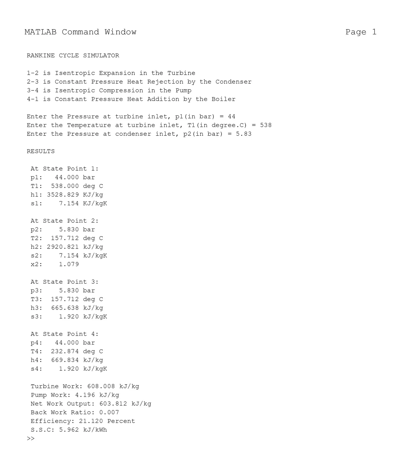
This section displays the results of the simulation, including properties of each state point, work interactions, efficiency, and specific steam consumption. Each result is printed with appropriate labels.

Output:

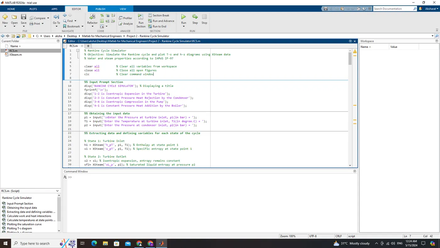
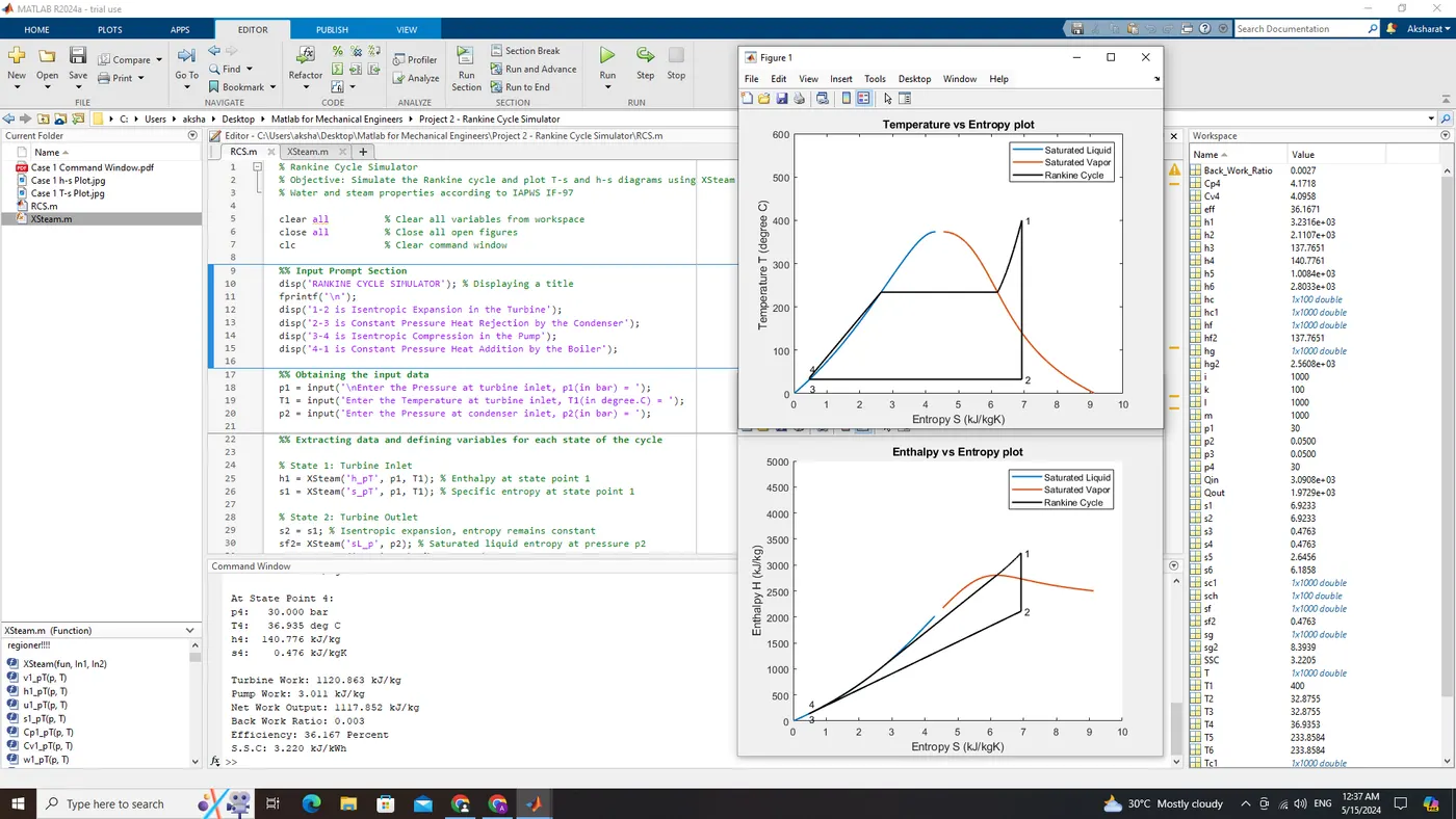
Case 1: Turbine Outlet is either Saturated state or Liquid-vapor mix state:

Pressure at Turbine Inlet (P1) = 30 bar

Temperature at Turbine Inlet (T1) = 400 deg Celcius

Pressure at Condenser Inlet (P2) = 0.05 bar

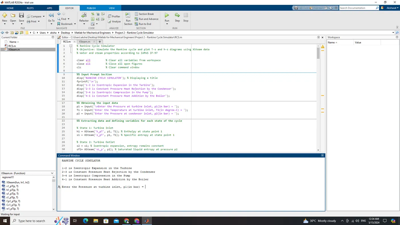
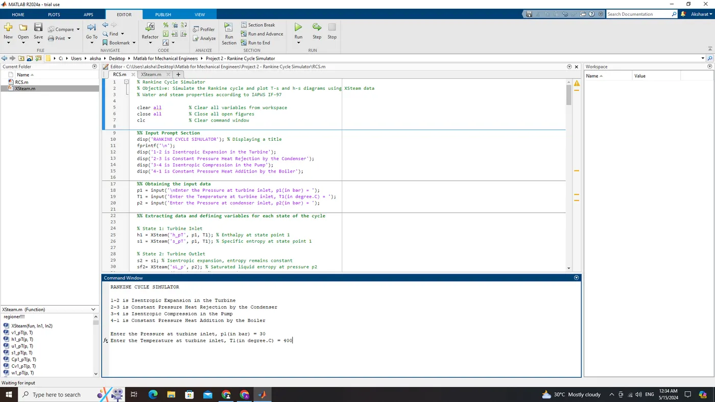
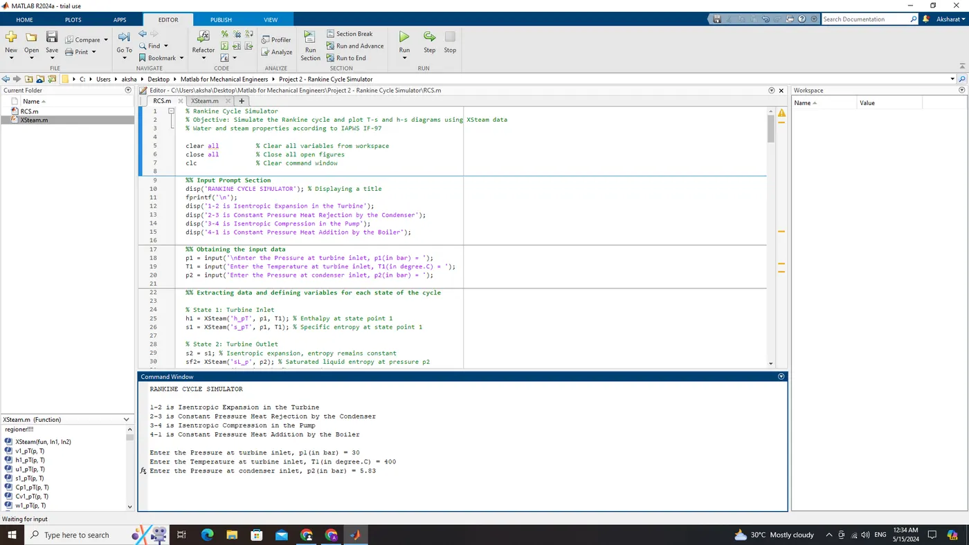
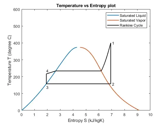
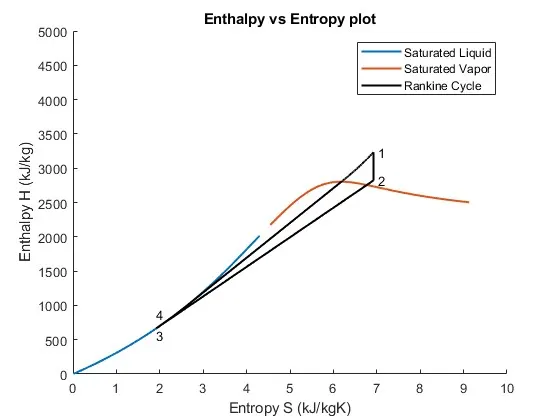
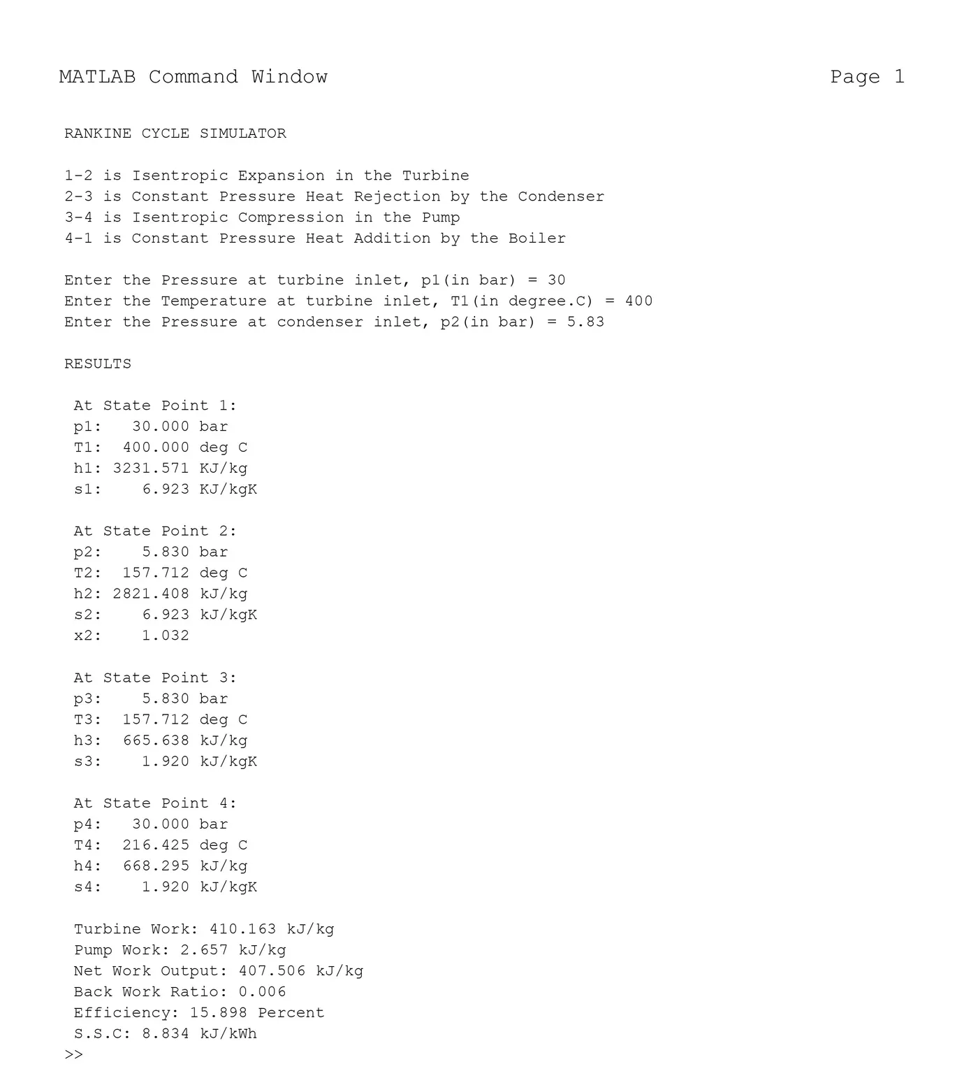
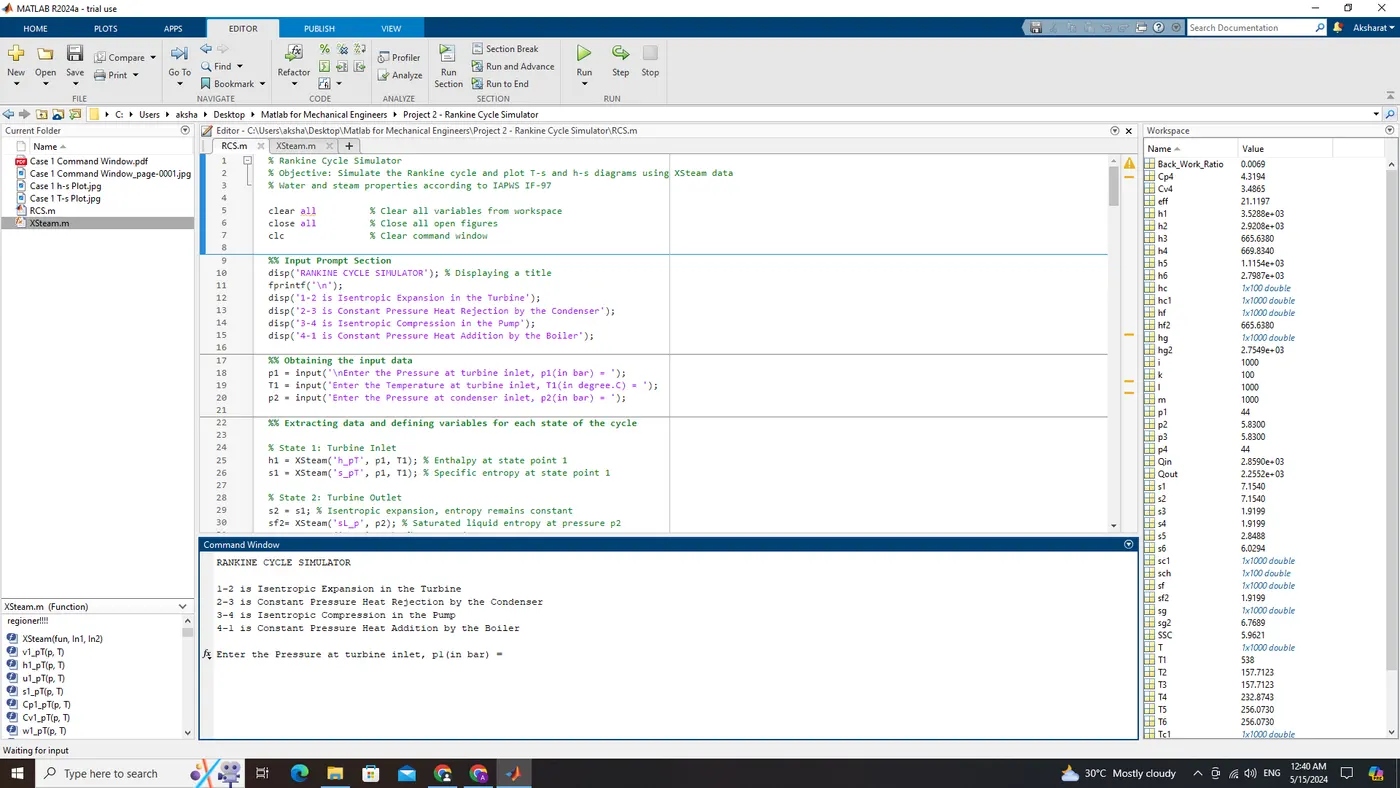
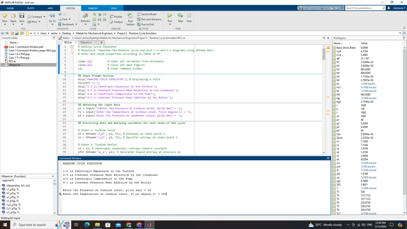
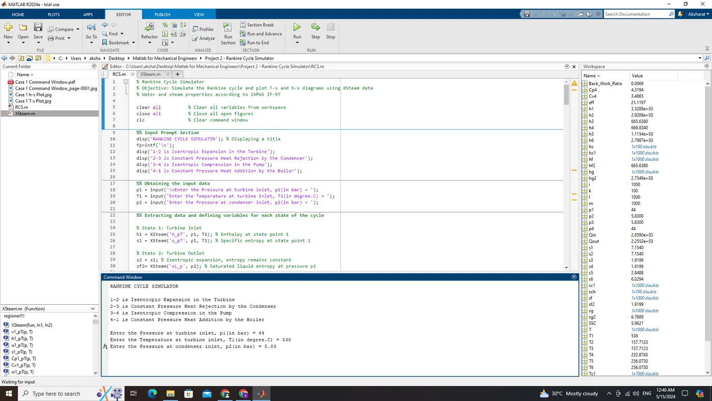
Case 2: Turbine Outlet is in Superheated state:

Pressure at Turbine Inlet (P1) = 44 bar

Temperature at Turbine Inlet (T1)= 538 deg Celcius

Pressure at Condenser Inlet (P2) = 5.83 bar

Conclusion:

In conclusion, the Rankine cycle simulator developed in MATLAB provides a comprehensive tool for analyzing thermodynamic processes within a Rankine cycle. Through meticulous calculation and visualization of state points, work interactions, and efficiency metrics, the simulator offers valuable insights into the performance of steam power generation systems. By leveraging XSteam data and adhering to IAPWS IF-97 standards, the simulator ensures accuracy in predicting cycle behavior under varying conditions. The T-s and h-s diagrams produced not only aid in understanding the cycle's thermodynamic properties but also serve as effective educational resources. Overall, this simulator serves as a practical and insightful tool for engineers, researchers, and students alike, facilitating the exploration and optimization of Rankine cycle-based energy systems.