Challenge

Project 2 - Rankine cycle Simulator

SSeenivasa Perumal21 Jul 2023

Rankine Cycle Process:

The Rankine cycle is a thermodynamic cycle that represents the idealized process of a steam power cycle used in steam power plants to generate electricity. It consists of four main processes, each of which involves specific changes in the thermodynamic properties of the working fluid (usually water and steam). Let's dive into each process and explain the terms involved:

1. Isentropic Expansion in Turbine (Process 1-2):

In this process, high-pressure and high-temperature steam from the boiler expands isentropically (reversible adiabatic process) in the turbine. The turbine extracts energy from the steam and converts it into mechanical work. Here are the terms involved:

Turbine: A device that converts the energy of a moving fluid (steam) into mechanical work through the principle of impulse or reaction. The turbine's rotor blades change the direction of the steam flow, and the kinetic energy of the steam is converted into rotational motion.
Isentropic Expansion: An isentropic process is an idealized, reversible adiabatic process with constant entropy. In an isentropic expansion, the steam expands without any heat exchange with the surroundings, and there is no increase in entropy.
Specific Enthalpy (h1): The total energy per unit mass of steam at the inlet of the turbine. It represents the sum of internal energy and flow energy (pressure energy) per unit mass.
Specific Entropy (s1): A measure of the amount of energy required to bring the steam to its current state. In an isentropic expansion, the entropy remains constant (s1 = s2).
Specific Enthalpy (h2): The total energy per unit mass of steam at the outlet of the turbine. It represents the sum of internal energy and flow energy (pressure energy) per unit mass.

2. Constant Pressure Heat Rejection in Condenser (Process 2-3):

After the steam expands in the turbine, it leaves the turbine at a lower pressure and temperature. The low-pressure steam is condensed at constant pressure in the condenser. Here are the terms involved:

Condenser: A heat exchanger where the low-pressure steam from the turbine is condensed into a saturated liquid. Cooling water or air is used to remove heat from the steam, causing it to condense.
Constant Pressure: The pressure in the condenser remains constant during the heat rejection process.
Specific Enthalpy (h2): The total energy per unit mass of steam at the inlet of the condenser. It represents the sum of internal energy and flow energy (pressure energy) per unit mass.
Specific Entropy (s2): A measure of the amount of energy required to bring the steam to its current state. The entropy at the end of the condensation process is higher than the entropy at the beginning due to heat transfer.
Saturated Liquid (h3): After condensation, the steam becomes a saturated liquid with the same pressure and temperature as in the condenser.

3. Isentropic Compression in Pump (Process 3-4):

The saturated liquid from the condenser is pumped to a higher pressure in the pump, preparing it for the next cycle in the boiler. Here are the terms involved:

Pump: A device that increases the pressure of the working fluid (liquid) by adding external energy to it. The pump provides the required energy to overcome the pressure difference between the condenser and the boiler.
Isentropic Compression: Similar to the isentropic expansion, an isentropic compression is an idealized, reversible adiabatic process with constant entropy. In an isentropic compression, the liquid is compressed without any heat exchange with the surroundings, and there is no increase in entropy.
Specific Enthalpy (h3): The total energy per unit mass of saturated liquid at the inlet of the pump. It represents the internal energy of the liquid.
Specific Entropy (s3): A measure of the amount of energy required to bring the liquid to its current state. In an isentropic compression, the entropy remains constant (s3 = s4).

4. Constant Pressure Heat Addition in Boiler (Process 4-1):

The high-pressure saturated liquid from the pump enters the boiler, where it is heated at constant pressure to become high-pressure steam. Here are the terms involved:

Boiler: A heat exchanger where the saturated liquid from the pump is heated to a high temperature by burning fuel (coal, natural gas, etc.) or using nuclear energy.
Constant Pressure: The pressure in the boiler remains constant during the heat addition process.
Specific Enthalpy (h4): The total energy per unit mass of steam at the outlet of the boiler. It represents the sum of internal energy and flow energy (pressure energy) per unit mass.
Specific Entropy (s4): A measure of the amount of energy required to bring the steam to its current state. The entropy at the end of the heating process is higher than the entropy at the beginning due to heat addition.

Rankine Cycle:

Formulas to Calculate Parameters:

Isentropic Efficiency (η_isentropic) of Turbine: η_isentropic = (h1 - h2s) / (h1 - h2), where h2s is the specific enthalpy at turbine outlet with isentropic expansion.
Work Done by Turbine (W_T): W_T = h1 - h2, where h1 and h2 are the specific enthalpies at turbine inlet and outlet.
Pump Work (W_P): W_P = vf * (p1 - p2) * 100, where vf is the specific volume of liquid at the condenser outlet.
Net Work Output (W_net): W_net = W_T - W_P
Heat Supplied (Q_s): Q_s = h1 - h4, where h4 is the specific enthalpy at the boiler exit.
Heat Rejected (Q_r): Q_r = h2 - h3, where h3 is the specific enthalpy at the condenser exit.
Thermal Efficiency (η): η = W_net / Q_s
Specific Steam Consumption (SSC): SSC = 3600 / W_net, where 3600 is used to convert work from KJ/Kg to KJ/KWh.
Back Work Ratio (BWR): BWR = -(W_P / W_T)

Code:

% Rankine cycle simulator

clear all 
close all
clc

disp('RANKINE CYCLE SIMULATOR')
disp('1-2 is isentropic expansion in turbine')
disp('2-3 is constant pressure heat rejection in condenser')
disp('3-4 is isentropic compression in pump')
disp('4-1 is constant pressure heat addition in boiler')

p1 = input('enter the pressure at the inlet of turbine (in bar) = ');
t1 = input('enter the temperature at the inlet of turbine (in degree Celsius) = ');
p2 = input('enter the pressure at the inlet of condenser (in bar) = ');

%Steam condition at the inlet of turbine
h1 = XSteam('h_pt', p1, t1);
s1 = XSteam('s_pt', p1, t1);

% Steam condition at the outlet of turbine
sg2 = XSteam('sV_p', p2);
sf2 = XSteam('sL_p', p2);
sfg2 = sg2 - sf2;
x2 = (s1 - sf2) / sfg2;
s2 = sf2 + x2 * sfg2;

hf2 = XSteam('hL_p', p2);
hg2 = XSteam('hV_p', p2);
hfg2 = hg2 - hf2;
h2 = hf2 + x2 * hfg2;

t2 = XSteam('Tsat_p', p2);

% Workdone by the turbine
W_T = h1 - h2;

%Steam condition at the outlet of condenser
p3 = p2;
t3 = XSteam('Tsat_p', p2);
h3 = XSteam('hL_p', p2);
s3 = XSteam('sL_p', p2);
vf = XSteam('vL_p', p2);
t22 = t3;

% Calculation of pump work
W_P = vf * (p1 - p2) * 100;

% Steam condition at state-4
p4 = p1;
h4 = W_P + h3;
s4 = s3;
t4 = XSteam('T_ph', p4, h4);

% Net workdone
W_net = W_T - W_P;

% Heat supplied
Q_s = h1 - h4;

% Heat rejected
Q_r = h2 - h3;

%Efficiency
efficiency = (W_net / Q_s);

% Specific steam consumption
SSC = 3600 / W_net;

tf_sat = XSteam('Tsat_p', p1);
sf_sat = XSteam('sL_p', p1);
hf_sat = XSteam('hL_p', p1);
sg_sat = XSteam('sV_p', p1);
hg_sat = XSteam('hV_p', p1);

%Plotting T-S diagram
hold on

% for plotting saturation curve
tsat1 = linspace(0, 374, 1000);

for i = 1:length(tsat1)
    ss1(i) = XSteam('sL_T', tsat1(i));
end

for j = 1:length(tsat1)
    ss2(j) = XSteam('sV_T', tsat1(j));
end

plot(ss1, tsat1, 'k', 'LineWidth', 2)
plot(ss2, tsat1, 'r', 'LineWidth', 2)

% for saturation temperature at p1
temp = XSteam('Tsat_p', p1);
t = linspace(t4, temp, 30);
for i = 1:length(t)
    S(i) = XSteam('s_pt', p1, t(i));
    hold on
end

t0 = linspace(temp, t1, 300);
for i = 1:length(t0)
    s0(i) = XSteam('s_pt', p1, t0(i));
end

% for plotting turbine work
plot([s1 s2], [t1 t2], 'g', 'LineWidth', 2)

% for heat rejection in condenser
plot([s2 s3], [t2 t3], 'b', 'LineWidth', 2)

% for pump work
plot([s3 s4], [t3 t4], 'r', 'LineWidth', 2)

% plotting curve line (constant pressure line in wet region) from outlet of
% the pump to the point from where phase change starts
plot(S, t, 'm', 'LineWidth', 2)

% Plotting the phase change region
plot([sf_sat sg_sat], [tf_sat tf_sat], 'b', 'LineWidth', 2)

% Plotting the curved constant pressure line from where the phase change
% ends to the superheated point
plot(s0, t0, 'm', 'LineWidth', 2)

legend('Saturation Curve L','Saturation Curve V','Turbine','Condenser','Pump','Boiler','location','northwest')
title('T-S Diagram')
xlabel('Entropy')
ylabel('Temperature')

%plotting H-S diagram
figure(2)
hold on

% for plotting the saturation curve
tsat1 = linspace(0, 374, 1000);

for i = 1:length(tsat1)
    hh1(i) = XSteam('hL_T', tsat1(i));
end

for j = 1:length(tsat1)
    hh2(j) = XSteam('hV_T', tsat1(j));
end

plot(ss1, hh1, 'b', 'LineWidth', 2)
plot(ss2, hh2, 'r', 'LineWidth', 2)

%for plotting turbine
plot([s1 s2], [h1 h2], 'g', 'LineWidth', 2)

%for condenser
plot([s2 s3], [h2 h3], 'b', 'LineWidth', 2)

%for plotting pump
plot([s3 s4], [h3 h4], 'r', 'LineWidth', 2)
s = linspace(s3, s1, 1000);

for i = 1:length(s)
    h(i) = XSteam('h_ps', p1, s(i));
end

%for plotting boiler
plot([s4 s1], [h4 h1], 'm', 'LineWidth', 2)
plot(s, h, 'c', 'LineWidth', 2)

legend('Saturation curve L','Saturation Curve V','Turbine','Condenser','Pump','Boiler','location','northwest')
title('H-S Diagram')
xlabel('Entropy')
ylabel('Enthalpy')

%Back work ratio
BWR = -(W_P / W_T);

%Output
% Saving the output to a text file
outputFileName = 'RankineCycleOutput.txt';
fid = fopen(outputFileName, 'w');

fprintf(fid, 'AT state point-1:\r\n');
fprintf(fid, 'p1 is : %.2f Bar\r\n', p1);
fprintf(fid, 'T1 is : %.2f Deg Celsius\r\n', t1);
fprintf(fid, 'H1 is : %.2f KJ/Kg\r\n', h1);
fprintf(fid, 'S1 is : %.2f KJ/KgK\r\n', s1);

fprintf(fid, '\r\nAT state point-2:\r\n');
fprintf(fid, 'p2 is : %.2f Bar\r\n', p2);
fprintf(fid, 'T2 is : %.2f Deg Celsius\r\n', t2);
fprintf(fid, 'H2 is : %.2f KJ/Kg\r\n', h2);
fprintf(fid, 'S2 is : %.2f KJ/KgK\r\n', s2);
fprintf(fid, 'X is : %.2f \r\n', x2);

fprintf(fid, '\r\nAT state point-3:\r\n');
fprintf(fid, 'p3 is : %.2f Bar\r\n', p3);
fprintf(fid, 'T3 is : %.2f Deg Celsius\r\n', t3);
fprintf(fid, 'H3 is : %.2f KJ/Kg\r\n', h3);
fprintf(fid, 'S3 is : %.2f KJ/KgK\r\n', s3);

fprintf(fid, '\r\nAT state point-4:\r\n');
fprintf(fid, 'p4 is : %.2f Bar\r\n', p4);
fprintf(fid, 'T4 is : %.2f Deg Celsius\r\n', t4);
fprintf(fid, 'H4 is : %.2f KJ/Kg\r\n', h4);
fprintf(fid, 'S4 is : %.2f KJ/KgK\r\n', s4);

% Additional calculations
fprintf(fid, '\r\nWork done by Turbine : %.2f KJ/Kg\r\n', W_T);
fprintf(fid, 'Work done by pump : %.2f KJ/Kg\r\n', W_P);
fprintf(fid, 'Heat added in the boiler : %.2f KJ/Kg\r\n', Q_s);
fprintf(fid, 'Heat rejected in the Condenser : %.2f KJ/Kg\r\n', Q_r);
fprintf(fid, 'Thermal efficiency : %.2f %%\r\n', efficiency*100);
fprintf(fid, 'Specific Steam Consumption : %.2f KJ/KWh\r\n', SSC);
fprintf(fid, 'Back Work Ratio : %.2f %%\r\n', BWR*100);

% Close the file
fclose(fid);

disp('Simulation results saved to RankineCycleOutput.txt');

Output:

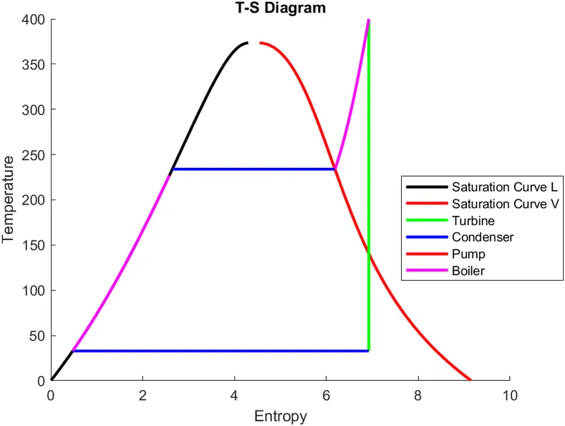
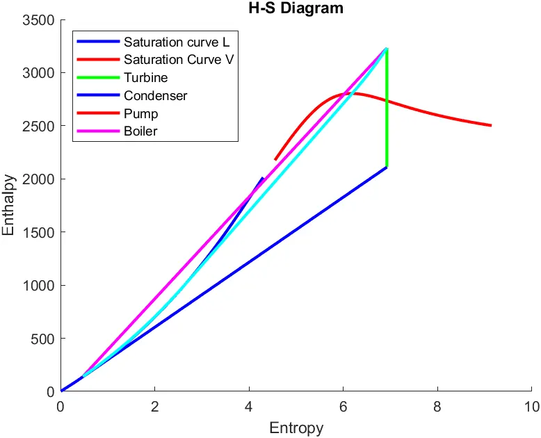
H-S Diagram:

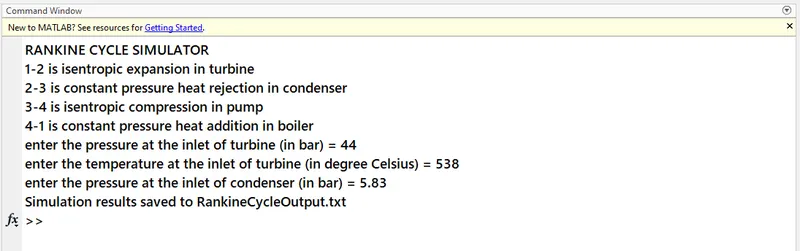
Output in Command Window:

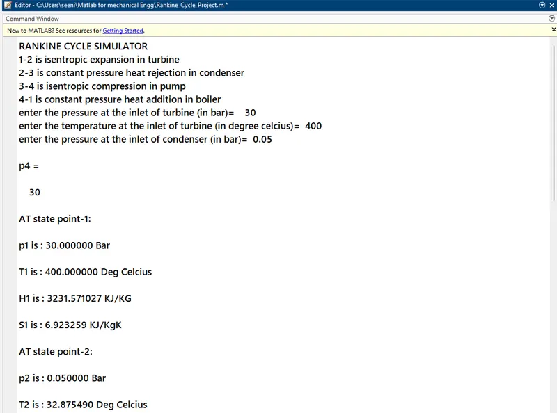
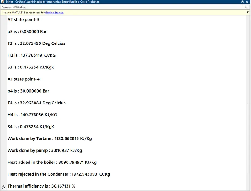
Command Window User Input:

ERROR AND REMEDIES :-

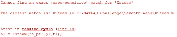
This error occurs due to incorrect name of saved file. As we know that, Matlab is a case sensitive, and if there have not matches a single words, it popup the error and thrown in the command window. For rectifying this error we need to make confirm written name in Matlab and file saving name in the same directory must be same otherwise, it showing same error.

This error occurs de to absent of parenthesis on either side. To solve this error we need to make confirm that, parenthesis must be on both the side. All the operator in matlab must be propar manner otherwise, it popup error in command window. This is due to MATLAB is a scientific programming language and it works on matrix.

Explanation of Code:

1. Introduction:

The Rankine Cycle Simulator is a MATLAB program that models an ideal Rankine cycle, a thermodynamic cycle commonly used in steam power plants. The Rankine cycle consists of four processes: isentropic expansion in the turbine (1-2), constant pressure heat rejection in the condenser (2-3), isentropic compression in the pump (3-4), and constant pressure heat addition in the boiler (4-1).

2. User Input: The simulator prompts the user to input the following parameters:
- Pressure at the inlet of the turbine (p1)
- Temperature at the inlet of the turbine (t1)
- Pressure at the inlet of the condenser (p2)

3. Turbine Inlet (State 1): The program calculates the thermodynamic properties (enthalpy and entropy) at the turbine inlet (state 1) using the provided pressure (p1) and temperature (t1) values.

4. Turbine Outlet (State 2): The program calculates the state 2 properties (enthalpy and entropy) at the turbine outlet assuming an isentropic expansion process (s2 = s1) and using the saturation properties at the condenser inlet pressure (p2). It determines the dryness fraction (x2) to differentiate between saturated liquid and vapor.

5. Condenser Exit (State 3): The simulator calculates the state 3 properties (enthalpy, entropy, and specific volume) at the condenser exit using the saturation temperature at pressure p2.

6. Pump Outlet (State 4): The program calculates the properties at state 4 (pump outlet) by assuming an isentropic compression process (s4 = s3). It determines the enthalpy (h4) using the work done by the pump (W_P) and the enthalpy at state 3 (h3).

7. Work Calculation: The simulator calculates the work done by the turbine (W_T) using the enthalpies at states 1 and 2. It also calculates the work done by the pump (W_P) using the specific volume (vf), pressure difference (p1 - p2), and a conversion factor.

8. Net Work and Heat: The program calculates the net work done by the cycle (W_net), which is the difference between the turbine work and pump work. It also calculates the heat supplied in the boiler (Q_s) and the heat rejected in the condenser (Q_r).

9. Efficiency and Specific Steam Consumption: The simulator calculates the efficiency of the Rankine cycle using the formula: efficiency = W_net / Q_s. It also computes the specific steam consumption (SSC) in kg/kWh using the formula: SSC = 3600 / W_net.

10. T-S and H-S Diagrams: The program plots the T-S (Temperature-Entropy) and H-S (Enthalpy-Entropy) diagrams of the Rankine cycle using MATLAB's "plot" function. The diagrams represent the various processes in the cycle and help visualize the thermodynamic changes.

11. Back Work Ratio (BWR): The simulator calculates the Back Work Ratio, which is the ratio of the pump work to the turbine work, using the formula: BWR = - (W_P / W_T).

12. Output: The program displays the results of the simulation, including the state points (pressures, temperatures, enthalpies, and entropies) and various calculated parameters (work, heat, efficiency, SSC, and BWR). It also informs the user that the simulation results have been saved to a text file named "Rankine_Cycle_Output.txt".

Overall, the Rankine Cycle Simulator is a powerful tool to understand and analyze the behavior of an ideal Rankine cycle and its various thermodynamic properties. The T-S and H-S diagrams provide visual insights into the cycle processes, and the output results can be saved and documented for creating a comprehensive project report on Rankine cycles and steam power plants.

Conclusion:

The Rankine cycle is a fundamental thermodynamic cycle used in steam power plants to generate electricity efficiently. Through simulation and calculations, we can determine various performance parameters such as net work output, efficiency, heat supplied and rejected, and back work ratio. The Rankine cycle plays a crucial role in understanding and optimizing power generation systems. By studying the Rankine cycle, engineers can design and improve power plants, leading to more efficient and sustainable energy production.

Reference:

https://en.wikipedia.org/wiki/Rankine_cycle#The_four_processes_in_the_Rankine_cycle

Drive Link:

https://drive.google.com/drive/folders/1u0x_Qd2jdIQ2BrIuwGyIFOGa3sdazSaD?usp=drive_link

Project 2 - Rankine cycle Simulator

Ship work like this
in your own course.

Talk to a career counsellor

Ship work like thisin your own course.

Talk to a career counsellor

Ship work like this
in your own course.