Project 2 - Development of TFT Cluster Speedometer Software Component

Introduction:

LCD based TFT cluster has become a norm in today's automotive market. Cluster comes with a 7 inch TFT LCD screen & a 32 bit micro controller. The Cluster could process various informations from other ECU's & display it in its large TFT LCD screen.

Architecture of the System :

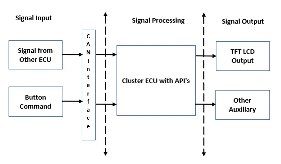
Cluster Instrument receives the signals from other ECU's via CAN bus interface. It also receives commands from the driver via steering wheel buttons. The signals are then processed by the Cluster ECU, after which the Cluster ECU may send the vehicle information to the LCD or light the LEDs and so forth, according to the results. Therefore, the Cluster ECU can be viewed as a carrier of the information flow.

The diagram below shows the overview of the system.

Signal Data :

All the signals involved in the model is shared in the following table-

SWC Name (Subsystem Name)	TFT_Cluster_Speedmeter_SWC
Sub SWC's Name	Sensor_Signal_Processing TFT_Display_Speed_Value_Control
Sampling Rate	10 ms (0.01 s)

Input Signal Name	Data Type	Min - Max Range	Signal Resolution	Description
In_MainFilt_SpeedValue	uint8	1 - 3	1	Main Filter Data for Speed Value Processing
In_AuxillaryFilt_SpeedValue	uint8	1 - 3	1	Auxillary Filter Data for Speed Value Processing
Avg_VehicleSpeed	uint16	0 kmph - 280 kmph	0.01 kmph	Local Variable for Average Vehicle Speed
Timer Input	uint16	0 - 3000	1	Input Timer
Output Signal Name	Data Type	Min - Max Range	Signal Resolution	Description
Out_VehicleSpeedDisplay	uint16	0 kmph - 250 kmph	0.01 kmph	Vehicle Speed displayed by Speedmeter
Local Signal Name	Data Type	Min - Max Range	Signal Resolution	Description
DisplaySpeed	uint16	0 kmph - 250 kmph	0.01 kmph	Display Speed Calculation
DisplaySpeed1	uint16	0 kmph - 280 kmph	0.01 kmph	Display Speed Calculation 1
DisplaySpeed_Filter	uint16	0 kmph - 280 kmph	0.01 kmph	Display Speed Filter Value
Averaging_output	uint16	0 kmph - 280 kmph	0.01 kmph	Output of averaged vehicle speed value

Functional Requirements and Simulink model:

The software component has four functional requirements to model. Each of them is described below.

1. Calculating TFT Display Speed :

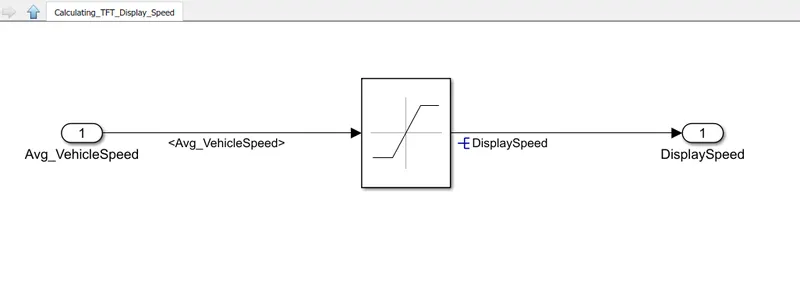
• Average Vehicle Speed would be displayed only if its between 2 kmph & 250 kmph. Any value outside this range will be discarded by its lower limit & upper limit.

• When Average Vehicle Speed is < 2 kmph, DisplaySpeed = 2 kmph.

• When Average Vehicle Speed is in between 2 kmph & 250 kmph, Display Speed = Average Vehicle Speed.

• When Average Vehicle Speed is > 250 kmph, Display Speed = 250 kmph.

This set of requirements is implemented using the saturation block. The signal Average_VehicleSpeed is passed through the saturation block which is configured to have upper limit of 250 and lower limit of 2. The output of the saturation block is the signal Display_Speed.

The block diagram is shown below.

2. Main Data Filtering:

• Main Data Filtering subsystem will be activated for every 10th millisecond.

• DisplaySpeed1 (t) = ((DisplaySpeed (t) x 0.65)/ Main Filter Speed Value) – 0.05

This subsystem is constructed as below.

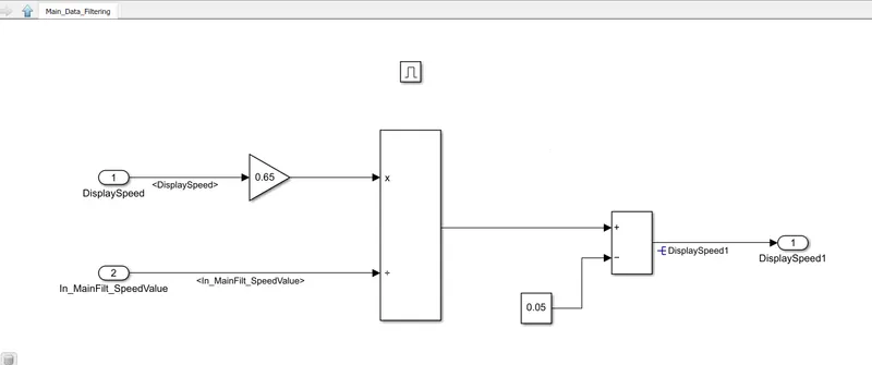
This is a enabled subsystem. The subsystem gets activated only when the control signal at enable port is high.

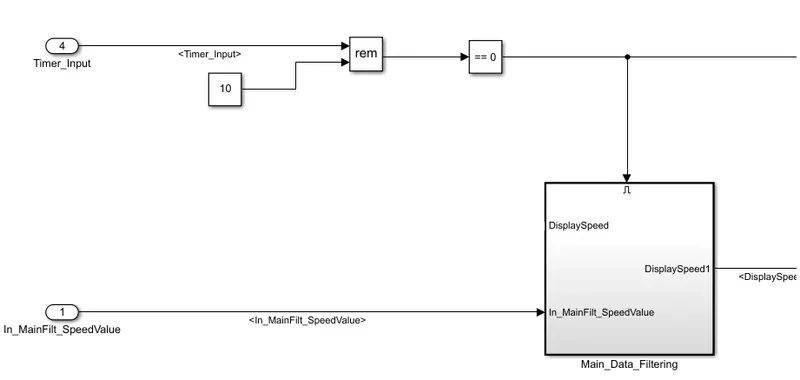
The control signal is generated by equating the remainder of timer input on dividing by 10, with 0. Meaning that every 10^th milisecond , the remainder will equal to 0 and the control signal will be high which will enable the main data filtering subsystem.

3. Auxiliary Data Filtering:

• Auxiliary Data Filtering subsystem will be activated for every 10th millisecond.

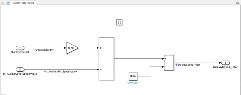
• DisplaySpeed_Filter (t) = ((DisplaySpeed1 (t) x 0.78)/ Auxillary Filter Speed Value) – 0.03

This subsystem is also modeled as enabled subsystem. The same control input is used for the enable port. The block diagram is shown below-

4. TFT Speed Output:

The condition to implement is this subsystem is stated as -

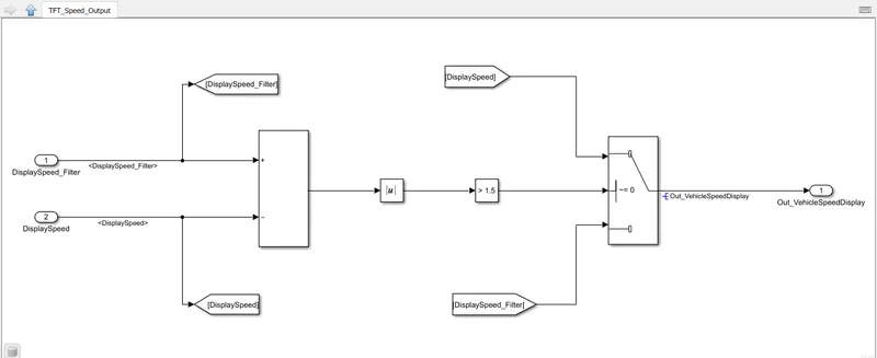
• If (DisplaySpeedFilter - Displayspeed)l > 1.5

{

Vehicle Speed Display = DisplaySpeed

}

else

{

Vehicle Speed Display = DisplaySpeed Filter

}

The above conditions are implemented using sum, abs, compare to constant and switch block. To ease the signal routing Goto tags are also used. The finished subsystem is shown in the following figure-

With all the subsystems modeled, we get final model. The completed model is shown below-

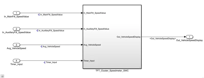
fig. top level of the model

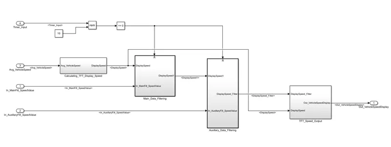
fig. connection of all subsystem

SLDD Creation:

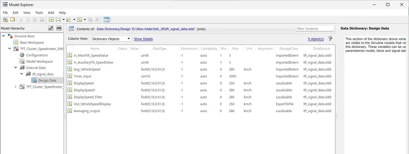
A data dictionary file is created. All the signals such as input, output and the local signals are added in the Simulink data dictionary.

The following image shows signals in the Sldd file.

Requirement Tagging:

Requirement tagging is done using the Requirement Manager app. At first the app is launched within the Matlab environment. Then we open the requirement editor and add new requirement set using the plus button in the top ribbon.

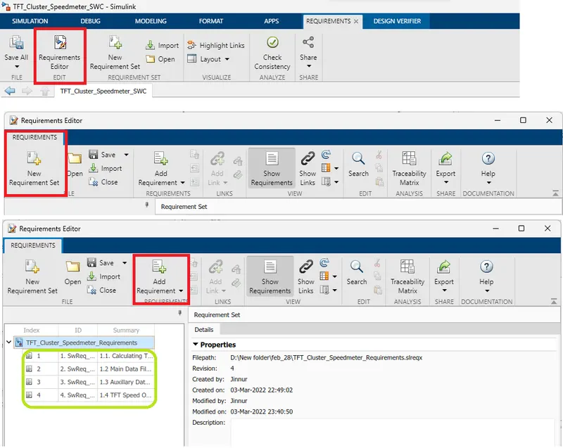
After the requirement set added, we can add requirements to that particular set. Here, we have created a set and added the four requirements to that set. A file with extension slreqx is generated after the requirement set is added.

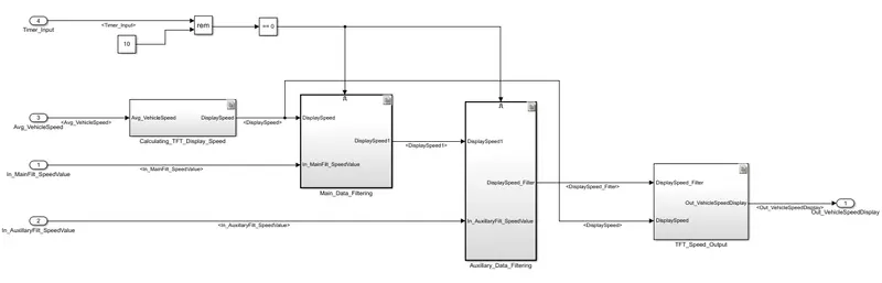
Then, each requirement is linked with the subsystem of the model where it is implemented. The subsystem in the simulink model is selected first, then in the requirement editor window particular requirement is linked with the ‘Add Link’ on the top. After we link all the subsystems, the model is shown in the figure below.

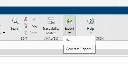
Now the requirement report is generated in word document format.

JMAAB Checks:

Then the model is check for JMAAB compliance. The model advisor tool is loaded and JMAAB checks were selected. Then checks were run and a report is generated.

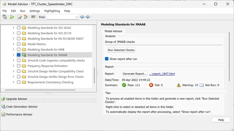
The model has passed 111 checks out a total of 125 checks and 14 warnings. An html report is also generated.

Simulink Design Verifier:

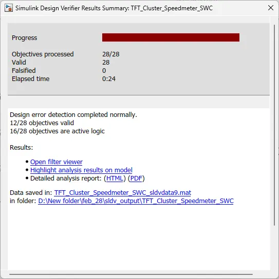
In the Simulink design verifier, we check the model for any design errors that may slipped through from the previous checks(i.e. jmaab). The design verifier tool is loaded from the App section.

Now we check for design errors by clicking green play button at the top. After few seconds the detection is completed and a report is also generated. Here is the summary of the verifier-

SLDV Test Generation report:

In the next step, test geneartion is done in the Design verifier tool. The test generation coverage is set to MCDC and other settings were left at default value.

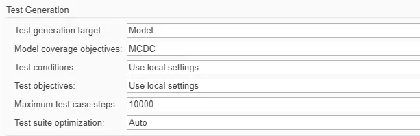
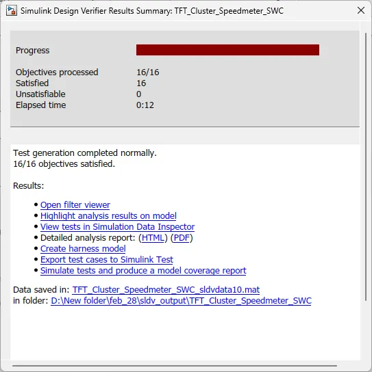
By clicking the run button the tests were generated and a html report is also created.

Model in Loop test + coverage:

Before going in to Model in loop testing the few configuration setting settings were taken care of such as Enabling coverage and setting Coverage metrics to MCDC.

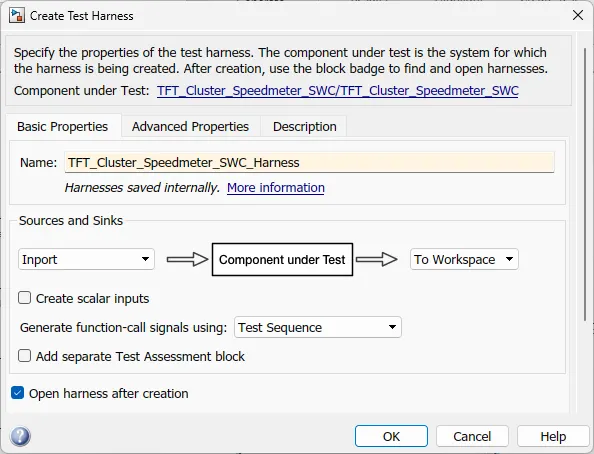
Now to test the model first we need a test harness. The test harness can be created by right clicking on the top level subsystem and selecting ‘Test Harness ’ from the context menu. This opens a dialogue box, where we can select the input and output of the component or model under test. Here we have selected signal builder for input and to workspace block for the output. The figure below shows the dialogue box parameters used-

Now, test cases were written for the model. They are written in a spreadsheet and then imported to the signal builder in test harness. A screenshot of the test cases is shown below-

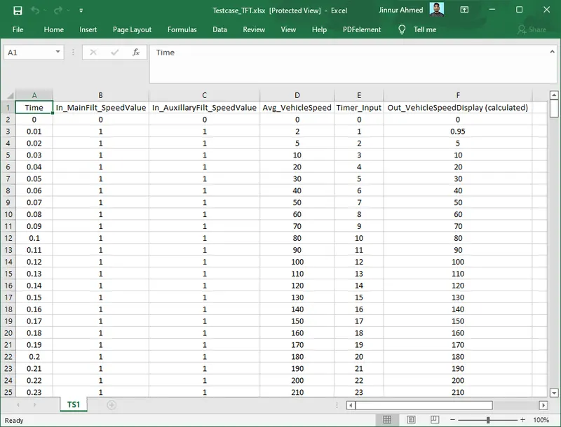
This data is then imported to the signal builder using the import form file option. Both the calculated output and the model output is send to workspace using ‘To Workspace’ block. These two workspace variables will be compared after the test.

So,the final model of the harness looks like the fig. below-

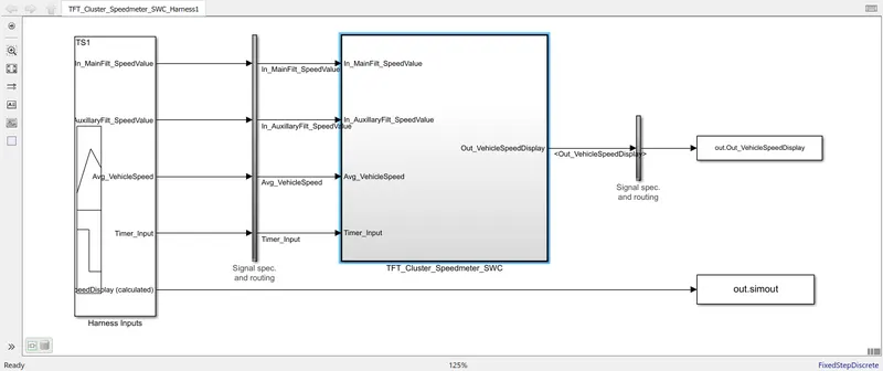
The model is then run for the total time of 1 sec with fixed step(discrete) solver with sample time of 0.01 sec. The output from test is then compared with the calculated value using the data inspector tool.

After we have run the model, the here is the comparison graph-

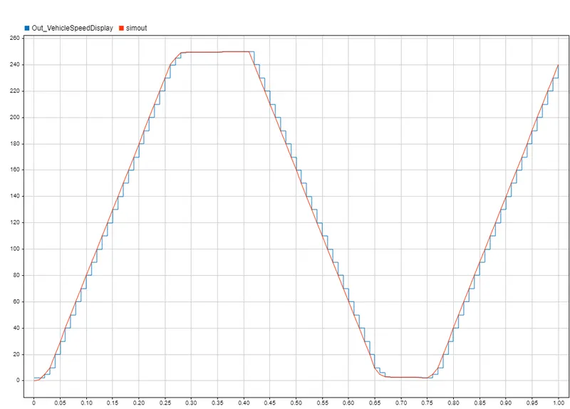
Here, the red graph is the manually calculated values and blue one is the output of the model. So, the model output closely follows the calculated one with very minimum deviations.

Coverage Report: Now, coming to the coverage analysis, the model has achieved full coverage in the test. The coverage report is generated and saved in the working folder.