Project 2
Pre-Processing:
- A MATLAB script has been created "Project2_init_file" to load all the variables needed to run and post-process the Simulink model.
Drive cycle selection is also done from here. Before running the Simulink vehicle model, the script is initialized at MATLAB to load all the variables in the workspace.
%%%%%%%%%%%%%%%%%%%%%%%%%%%%%%%%%%%%%%%%%%%%%%%%%%%%%%%%%%%%%%%%%%%%%
%% Skill-Lync -> Hybrid Drives Development
% Project 1 - Conventional Vehicle Model
% By - Sri Harsha Avvari
% Description:
%% Initialization File
% Initialization file for loading the variables for the Conventional vehicle simulation model
%% Vehicle Parameters
M = 1500; % Vehicle weight [kg]
Cr = 0.015; % Rolling resistance coefficient
Rw = 0.35; % Rolling radius [m]
Cd = 0.33; % Drag coefficient
Af = 2; % Frontal area [m2]
rhoa = 1.225; % Air density [kg/m3]
Vwind = 0; % Wind velocity [kmph]
g = 9.81; % Gravitational acceleration [m/s2]
theta = 0; % Slope [deg]
myu_road_tire = 1; % Coefficient of friction between tire - road interface
%% Powertrain Parameters
FDR = 3.73; % Final Drive Ratio / Diff Ratio
DiffEff = 0.99; % Differential efficiency (assumed independent of operating conditions)
NumGear = 4; % Number of gears in transmission
TransGear = [1:NumGear]; % Transmission Gears
TransRatio = [3.06, 1.62, 1, 0.7]; % Corresponding Transmission ratios
TransEff = 0.90; % Transmission efficiency (assumed independent of operating conditions)
TC_SR = [0, .5, .6, .7, .8, .87, .92, .94, .96, .97, 1]; % Torque Converter Speed Ratio (Matlab default) -> TurbSpd/PumpSpd
TC_TR = [2.232, 1.5462, 1.4058, 1.2746, 1.1528, 1.0732, 1.0192, 1, 1, 1, 1]; % Torque Converter Torque Ratio (Matlab default) -> TurbTrq/PumpTrq
TC_Cf = 1e-4 * [.72558, .66322, .63463, .59042, .51331, .4144, .29287, .22444, .12186, .04386, 0]; % Torque Converter Capacity Factor (Matlab default) -> PumpTrq/PumpSpd^2 [Nm/rpm^2]
load Vehicle_Data/Engine_data_1_9L_Saturn_95kW
load Vehicle_Data/Trans_Shift_map
load Vehicle_Data/EM_Honda_Insight_10kW
load Vehicle_Data/ESS_NiMH6
ESS_init_soc = 0.8;
ESS_soc_max = 0.9;
ESS_soc_min = 0.6;
%% Driver Parameters
Kp = 10; % P gain for driver PI model
Ki = 1; % I gain for driver PI model
Drive_Cycle_Select = 1; % Drive cycle selection
% Drive cycle values in m/s
if Drive_Cycle_Select == 1
load DriveCycles/UDDS;
elseif Drive_Cycle_Select == 2
load DriveCycles/HWFET;
elseif Drive_Cycle_Select == 3
load DriveCycles/FTP;
elseif Drive_Cycle_Select == 4
load DriveCycles/US06;
elseif Drive_Cycle_Select == 5
load DriveCycles/NEDC;
elseif Drive_Cycle_Select == 6
load DriveCycles/WLTP;
end
time_end = cyc_time(end);
vel_end = cyc_vel(end);
- The Drive Cycle can be selected from this MATLAB Script, By changing the variable Drive _Cycle _Select to,
- UDDS
- HWFET
- FTP
- USO6
- NEDC
- WLTP
Simulink modeling:
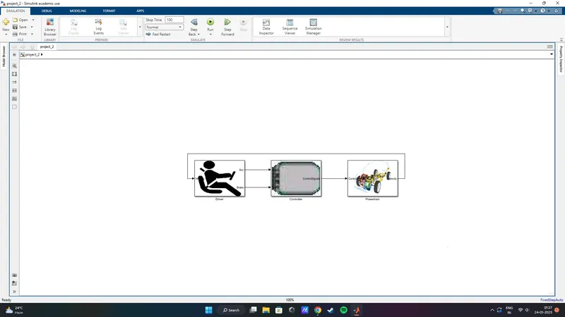
The vehicle design mainly consists of three parts Driver, Controller and the Powertrain.
Driver:
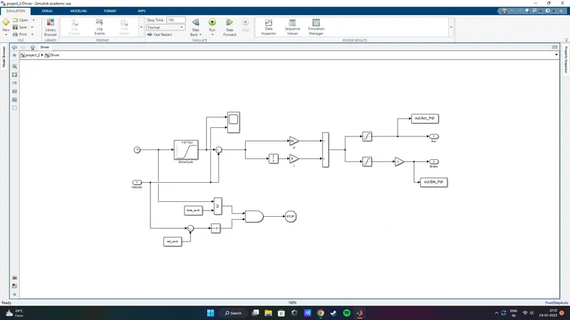
The Driver model shown is a basic PI controller that generates accelerator and brake pedal outputs to match the desired and actual vehicle speeds.
CONTROLLER:
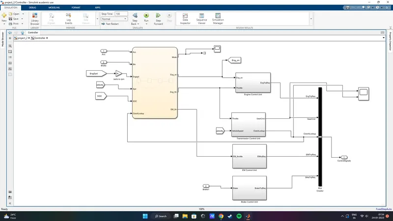
The controller is the brain of the vehicle which represents the electronic controls units, Based on the driver inputs it generates an engine torque, a transmission gear and a brake torque. These inputs are fed from supervisory controller to the control unit which is then fed to the powertrain which drives the vehicle.
A state flow chart is used for the supervisory control unit which decides the operating mode whether it is start /stop mode or cruising mode or regen braking mode for each modes the engine drive and the motor drive are controlled.
ENGINE CONTROL UNIT:
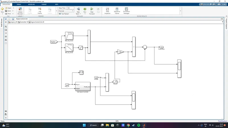
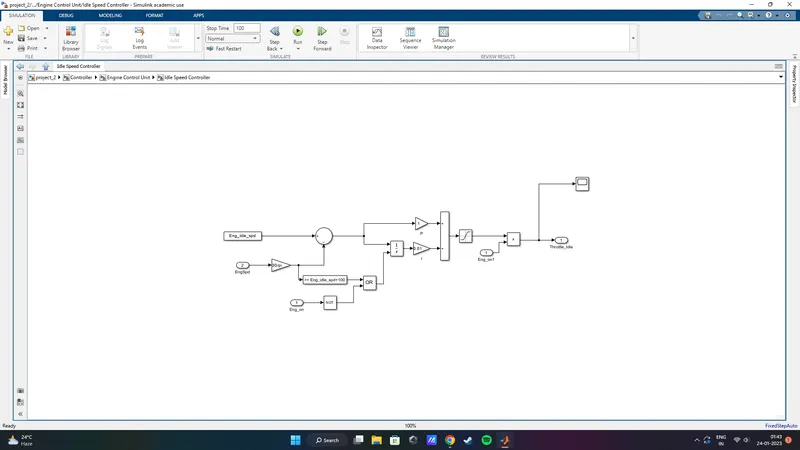
In the existing Engine Control Unit for the Conventional Vehicle, there are some changes made to be a Hybrid Drivetrain. New input signals are implemented like 'Eng_on'. The logic behind this is to make the Vehicle more Fuel efficient by turning off the engine whenever it is not required.
IDLE SPEED CONTROL UNIT:
TRANSMISSION CONTROL UNIT:
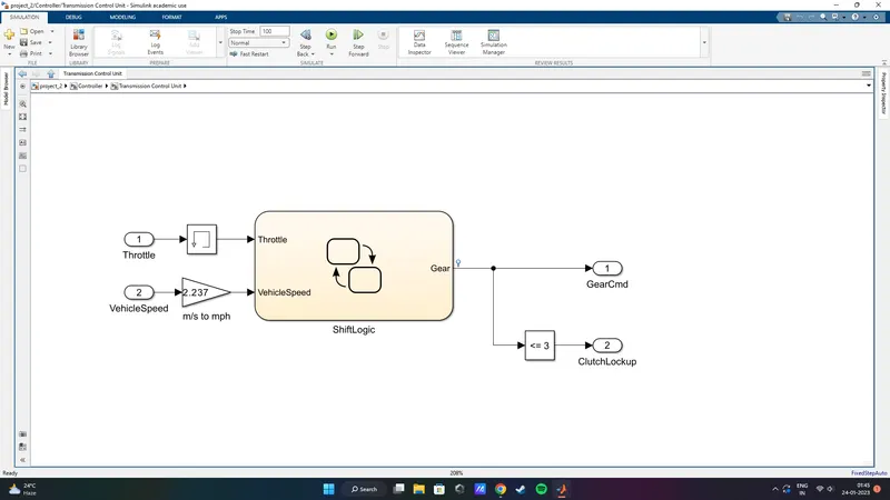
The transmission control unit is used to control the gear shifting using the study flow variable chart. The gear shifting is controlled according to the vehicle speed and throttle input, the gear command is passed to the transmission block to select the desired gear ratio.
EM CONTROL UNIT:
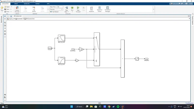
Motor control unit compare EM speed with the max torque curve and max torque generation curve of the lookup table and give the required torque command to the electric motor. EM Control Unit gives us 'EMTrqReq' which is Engine Machine Torque Requirement.
BRAKE CONTROL UNIT:
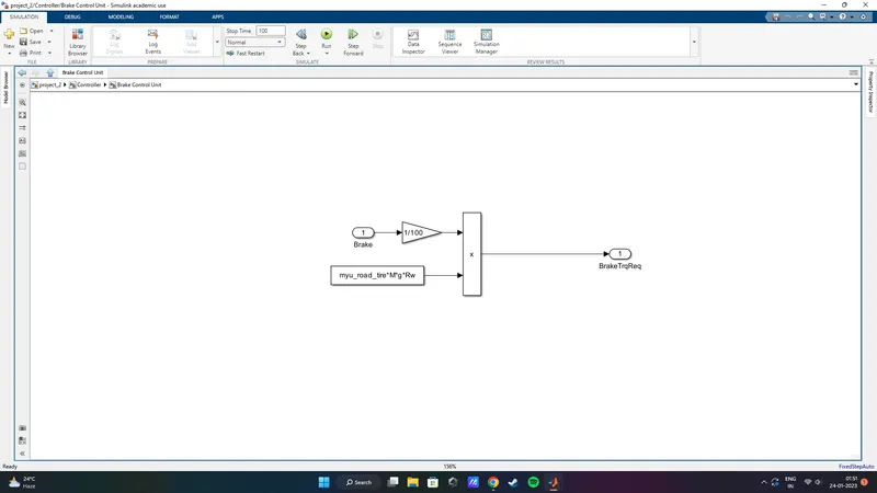
Brake control unit produce required brake torque according to the brake pedal input and passes the brake torque in to the wheel block in the transmission model.
POWERTRAIN UNIT:
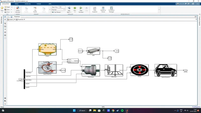
The power train unit has all the parts that transfer the power of the engine to get the vehicle in motion. This includes engine, electric motor, battery, transmission, differential, wheels, and vehicle body dynamics subsystem.
ENGINE:
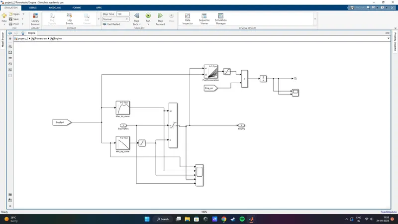
The engine speed is the input given based on which the required torque is generated by staurating the max torque curve and min torque curve and sends the reuired engine torque to the crank.
ELECTRIC MOTOR:
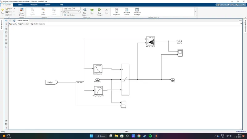
Engine speed is given as input which is then saturated between EM max torque curve and EM nax generating torque curve which gives us the EM torque which is then sent to the crank, Electric power is also generated.
BATTERY:
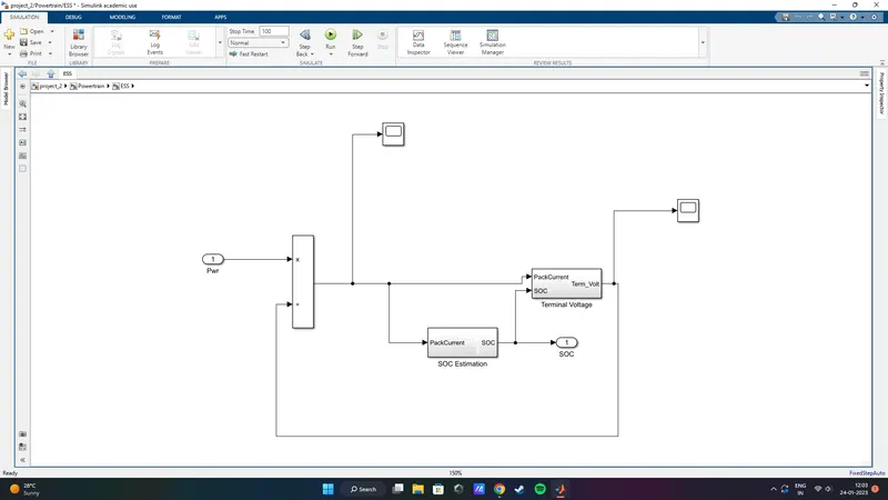
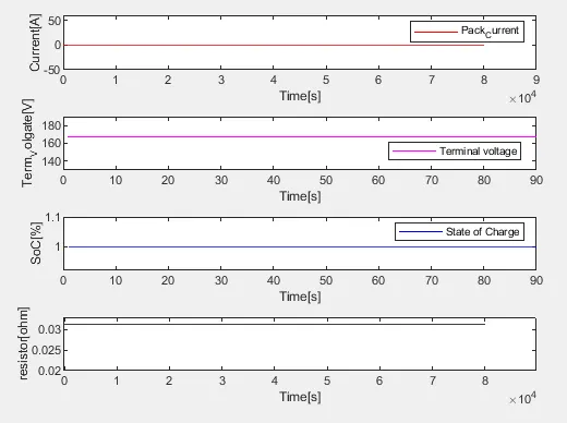
The input to Battery pack is electric power and battery soc is the output. two different subsystems have been created to determine the soc estimation and terminal voltage separately soc is used to determine the terminal voltage.
SOC ESTIMATION:
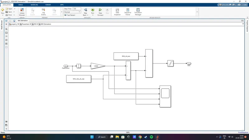
Pack current in ampere is converted to amp-hr and is divided with max capacity and added with the initial soc to determine the soc of the battery, at each instance the soc value is limited between 0 to 1.
TERMINAL VOLTAGE:
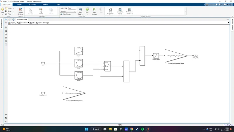
Input is Pack current and SOC and output is the terminal voltage,the Voltage drop is subtracted with an open circuit voltage and then multiplied with gain block to calculate the terminal voltage
CRANK:
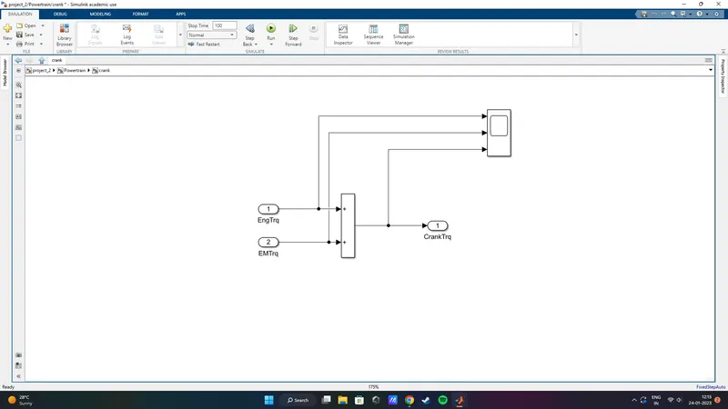
The crank hub adds the EM torque and the Engine torque to give the output as the crank torque which is sent to the transmission
TRANSMISSION:
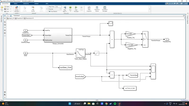
in this the input is crank torque, ClutchLockup and gear selector from controller signal for transmission of gear ratio. The ratio is multiplied by transmission input torque and then the transmission efficiency positive torque and negative torque gives transmission outputspeed.
TORQUE CONVERTER:
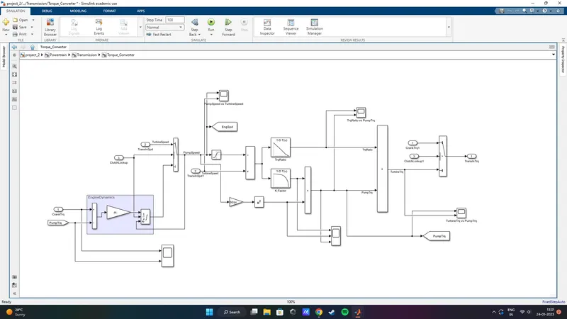
The gear selection from the transmission control unit is multiplied by the engine torque and the efficiency and engine dynamics of the torque converter are applied in this model.Torque converter defines the pump torque and turbine torque by the clutchLock up status, and the combination gives us the transmission torque.
DIFFERENTIAL:
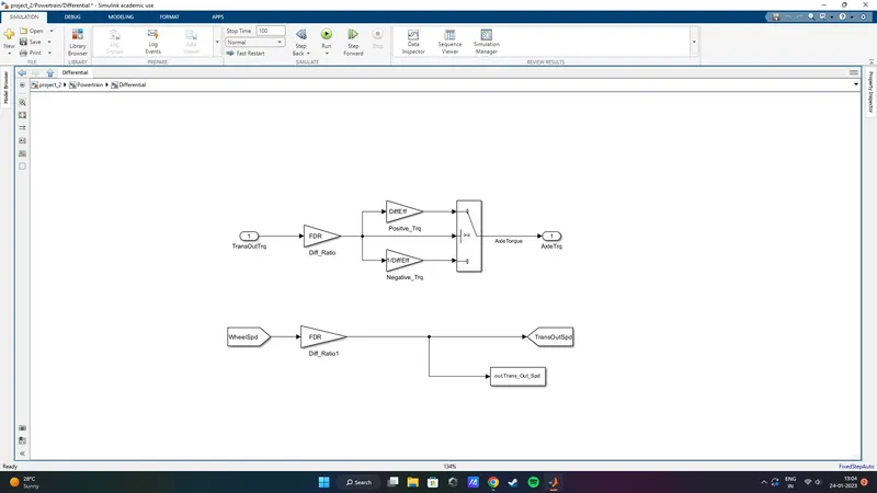
The TransOutTrq is the input which is multiplied by the differential ratio and differential efficiency and the obtained torque is transmitted to the wheels as the axle torque.
WHEELS:
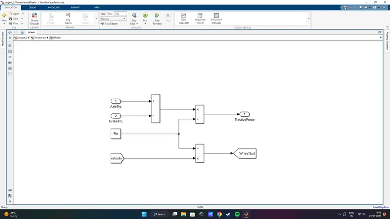
- The brake torque from the control model is subtracted from the Axle torque and divides from the rolling radius to determine the Tractive force.
- The Wheel speed is calculated from the vehicle velocity and saved in the workspace.
VEHICLE DYNAMICS:
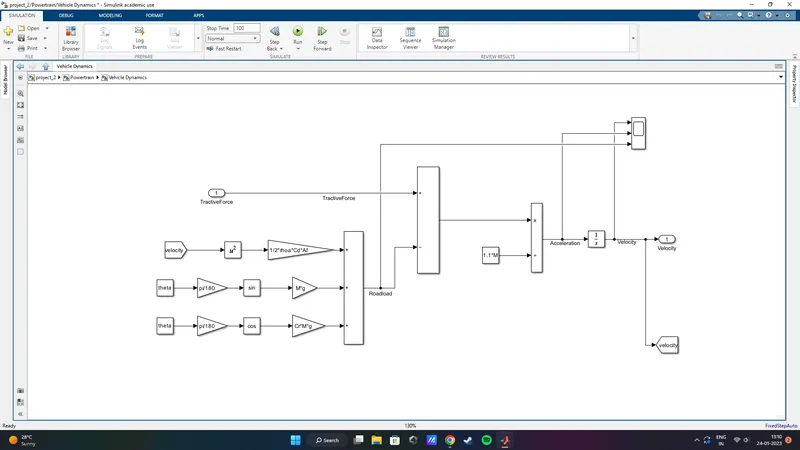
- The longitudinal dynamics of the vehicle along with the road load is represented in the 'Vehicle Dynamics' block.
- The Tractive force and the road load are used to calculate the vehicle acceleration and velocity.
The dynamic equation for designing the Vehicle dynamic block is

where,
p = air density [kg/m^3]
A = Frontal area [m^2]
Cd = drag Coefficiend
Vveh = velocity of vehicle [m/s^2]
Vwind = velocity of wind [m/s^2]
Cr = rolling resistance coefficient
M = mass in [Kg]
MATLAB code for post processing and plotting:
g = gravity.
PLOTS:
For UDDS:
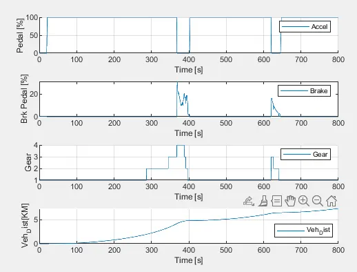
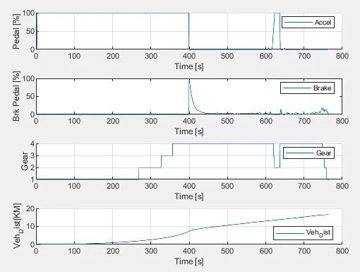
1] accelerator and brake pedal, gear command, and actual speed, vehicle distance.
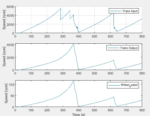
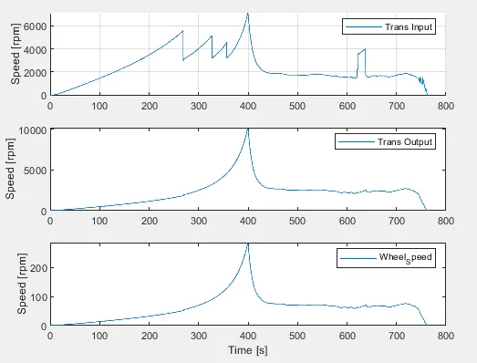
2] time trace for engine, transmission input, transmission output and wheel speed
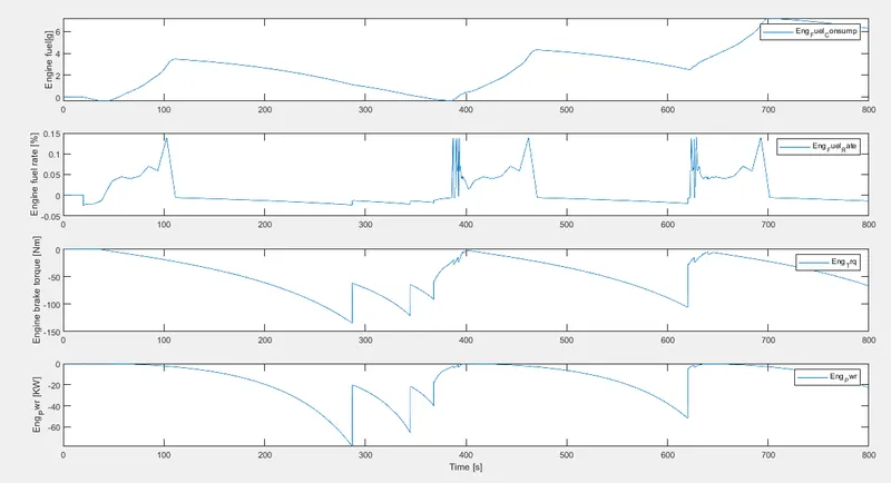
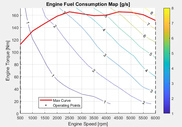
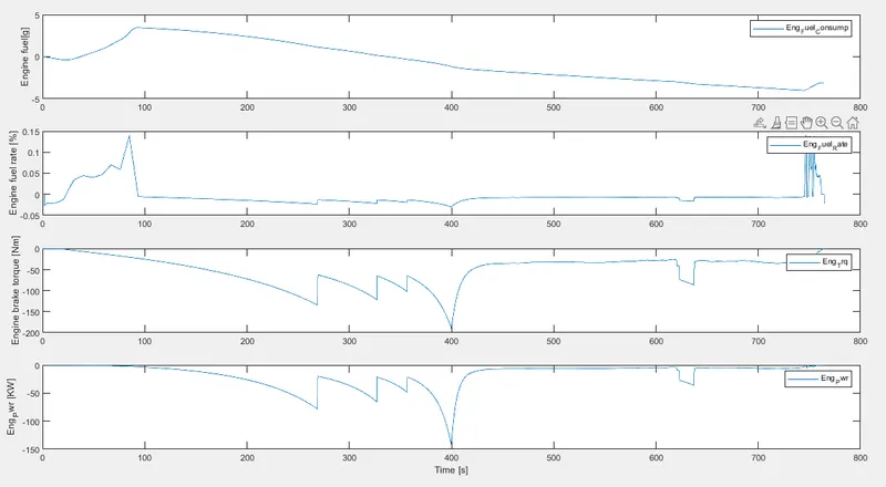
3] engine torque, engine power, fuel rate and fuel consumption.
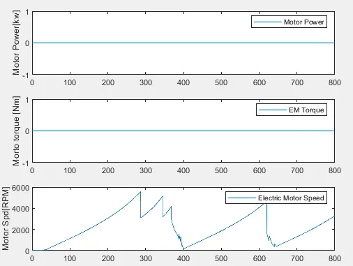
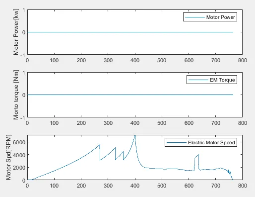
4] Motor power, Torque, Speed.
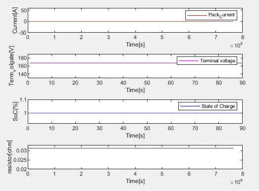
5]ESS Terminal voltage, Current, SOC, Resistor.
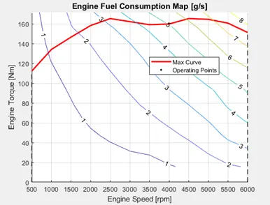
6]engine operating points on the engine fuel map.
For HWFET:
1]accelerator and brake pedal, gear command, and actual speed, vehicle distance
2]time trace for engine, transmission input, transmission output and wheel speed
3] engine torque, engine power, fuel rate and fuel consumption.
4] Motor power, Torque, Speed.
5] ESS Terminal voltage, Current, SOC, Resistor.
6] engine operating points on the engine fuel map.
Conclusion:
The modeling process of a forward energy-based fuel consumption model of a P1 Hybrid vehicle is designed in MATLAB using codes and simulink in MATLAB. All the required plots during UDDS and HWFET cycle were generated.All the Post-processing calculations were executed and the graphs were successfully plotted.