Challenge

Project 1

SSri Harsha Avvari10 Jan 2023

Main Aim of the project is to finish the tasks given:

a. Tabulate the fuel economy numbers (kmpl) for UDDS and HWFET cycle. This forms the baseline numbers for comparing with the future hybrid version.
b. Plot the time trace for engine, transmission input, transmission output and wheel speed on one plot.
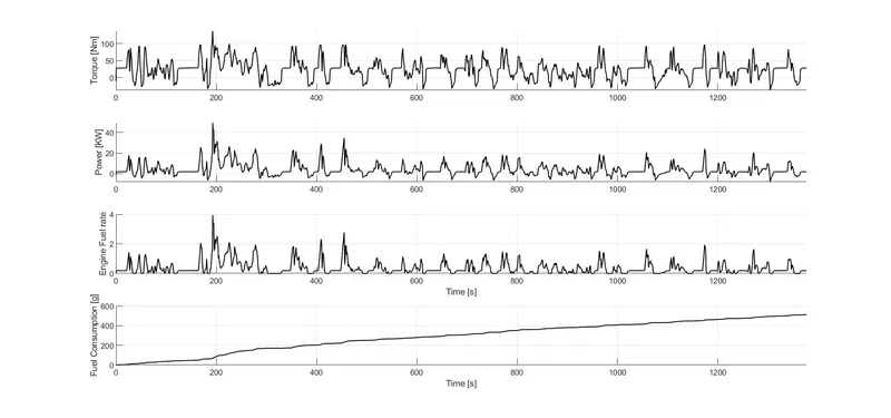
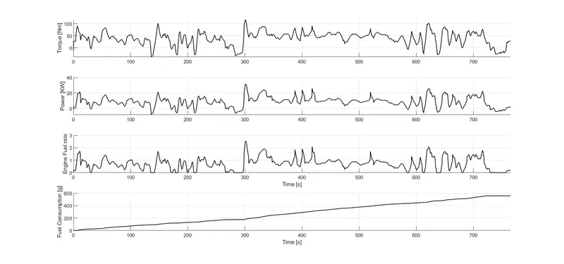
c. Plot engine torque, engine power, fuel rate and fuel consumption using subplots.
d. Plot accelerator and brake pedal, gear command, vehicle desired and actual speed, vehicle distance using subplots.
e. Plot the engine operating points on the engine fuel map.
f. Write down appropriate brief comments on each of these plots, describing the vehicle behavior throughout the drive cycle.
g. Generate the plots for both drive cycles

Forward-Modelling Approach

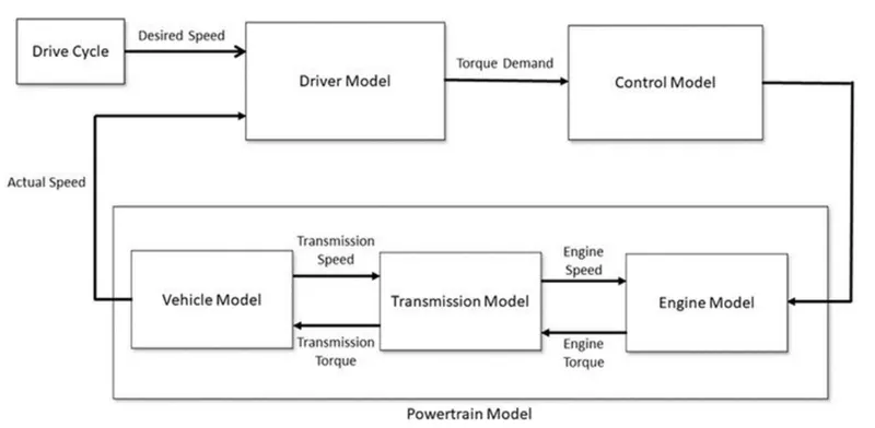
It also known as dynamic simulation. Dynamic models are used for detailed simulations. In this model force/torque/power is the input and the vehicle state variable velocity and acceleration are outputs. The models and simulatios are more realistic due to phhysical casualty hence appropriate for control development. There is feedback loop to meet the desired vehicle state. It is mainly used to simulate a vehicle on a driving cycle to analyse the dynamic behaviour of the system helps significantly in control development.

Architecture of the forward conventional vehicle model is presented in Figure:

Matlab script:

In this project, a typical midsize car with a 1.9L engine and a 4-speed automatic transmission is considered. Data is taken from ADVISOR data base developed by NREL, USA. Transmission shift map and controller is taken from Matlab/Simulink example database.

The model developed has the capability to simulate the vehicle on different drive cycles like UDDS, HWFET, FTP, NEDC, etc.

“Project1_InitFile.m” is a Matlab script used to load all the variables required for running the Simulink model and for post-processing. The drive cycle selection is also done here. Before running the Simulink vehicle model, run this initialization script.

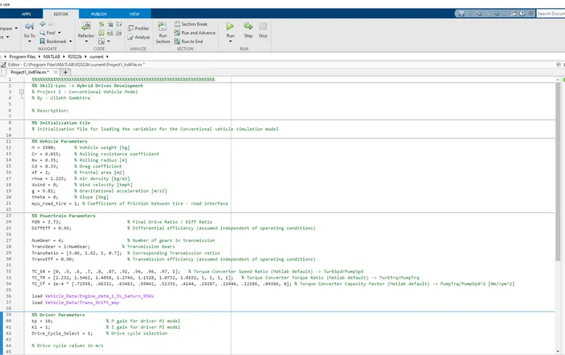
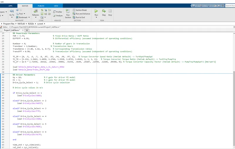
The Drive Cycle can be selected from this MATLAB Script, By changing the variable Drive_Cycle_Select to,

1	UDDS
2	HWFET
3	FTP
4	US06
5	NEDC
6	WLTP

lets see the simulink model of conventional vehicle,

The model developed has the capability to simulate the vehicle on different drive cycles like UDDS, HWFET, FTP, NEDC, etc.

Driver Model:-

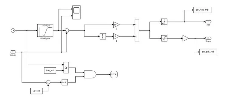
It is modeled using a ‘Driver’ block, which is a basic PI controller that generates accelerator and brake pedal outputs to match the desired and actual vehicle speeds.

Control Model:-

The ‘Controller’ block is the brains of the vehicle, representing the electronic controls units. It is based on the driver inputs, it generates desired engine torque, desired transmission gear and desired brake torque. These inputs are fed to the ‘Powertrain’ block which represents the drivetrain of the vehicle.

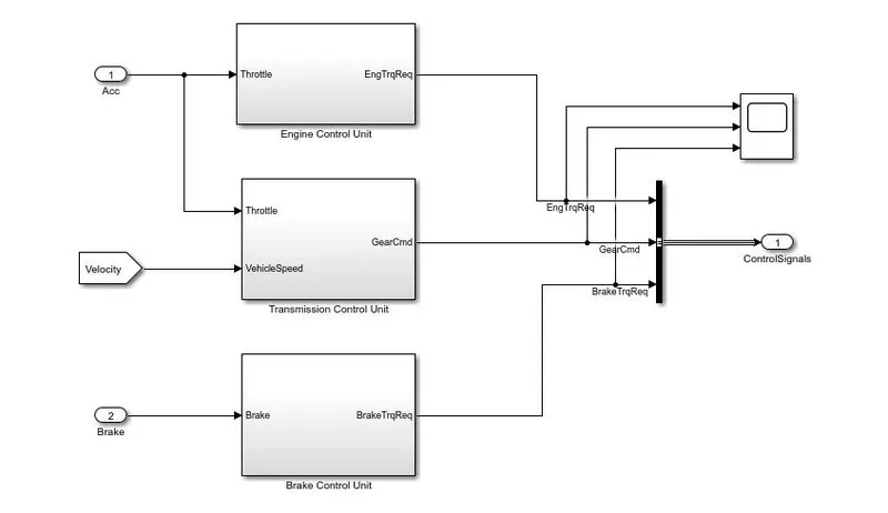
1] Engine control Unit:-

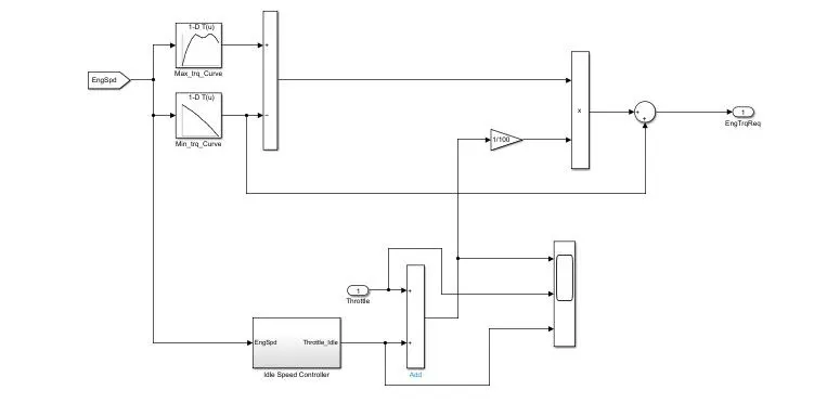
The input given is engine speed in an engine control unit and the output is the torque required for engine.

2] Transmission Control Unit:-

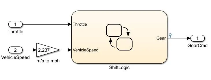
The shifting of gear is controlled according to the speed of vehicle and throttle input.

3] Brake Control Unit:-

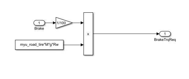
The brake torwue unit produces required brake torque depending on the input given to brake pedal and passes the feedback to the transmission model.

3] PowerTrain:-

The powertrain contains all the components that converts the engines power into motion.

1] Engine:-

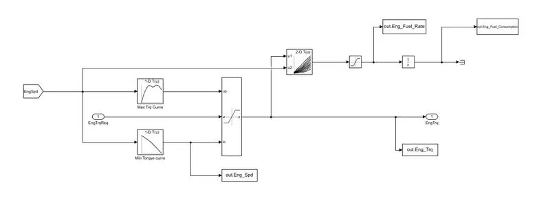
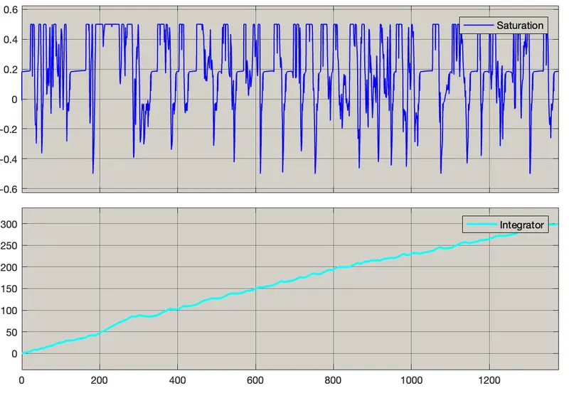
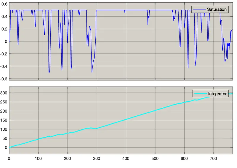
we have used a map based model to design the fuel consumption of engine. It is based on maximum Torque and minimum torque from the engine speed and then the torque is saturated which gives output engine torque, the saturated torque and engine speed map give fuel consumption output is saturated and is then integrated.

2] Transmission:-

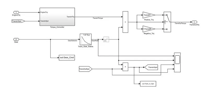
The engine block is connected to the automatic transmission via a torque converter. The output of the transmission is connected to the differential.

3] Differential:-

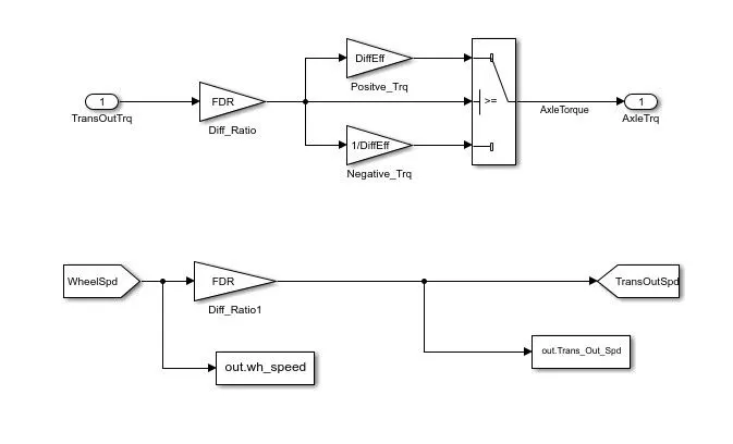
The transmission output torque is multiplied by the differential ratio and differential efficiency in this block and the torque is transmitted to the wheel as the axle torque.

4] Wheels:-

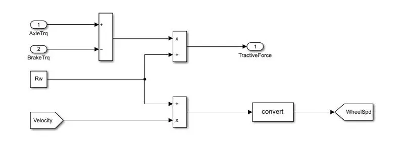
The brake torque from the control model is subtracted from the Axle torque and divides from the rolling radius to determine the Tractive force.
The Wheel speed is calculated from the vehicle velocity and saved in the workspace.

5] Vehicle Dynamics:-

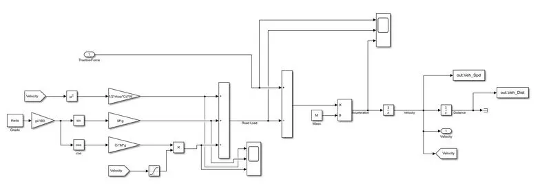
The longitudinal dynamics of the vehicle along with the road load is represented in the 'Vehicle Dynamics' block.

SIMULATION RESULTS:

UDDS cycle:

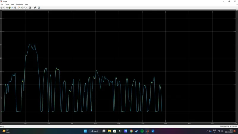
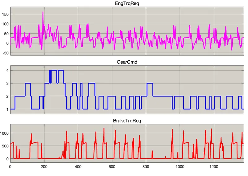
Engine Torque, Transmission Gear and Brake Torque :

Fuel Rate and Fuel Consumption :

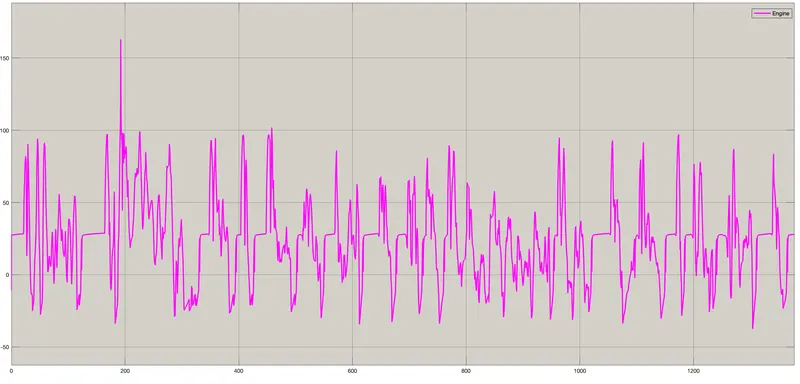
Engine Torque :

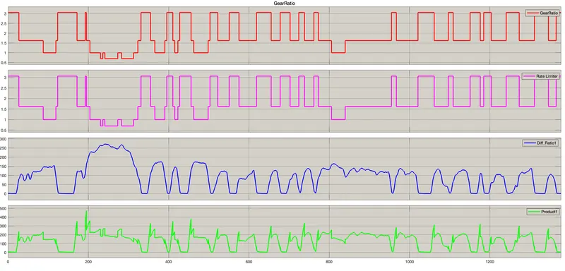
Gear Ratio, Trans Input and Output Speed :

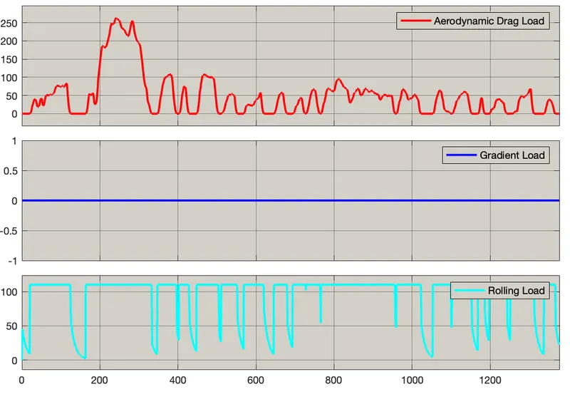
Types of road loads ( Aerodynamic drag load, gradient load and rolling load):

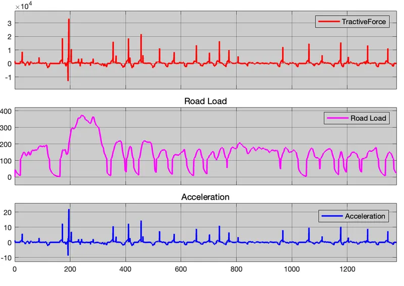
Tractive Force, Road Load and Acceleration :

2. HWFET Drive Cycle

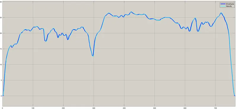
Drive Cycle and Actual Velocity :

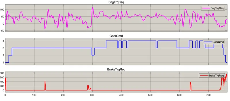
Engine Torque, Transmission Gear and Brake Torque during HWFET cycle:

Fuel Rate and Fuel Consumption :

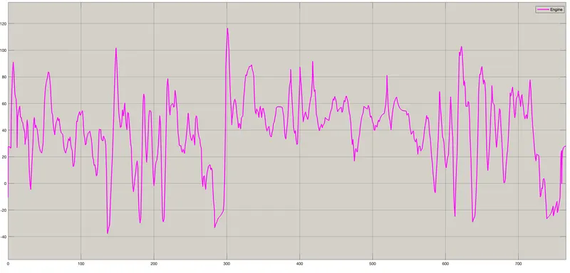
Engine Torque :

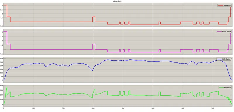
Gear Ratio, Trans Input and Output Speed :

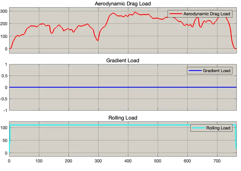
Types of road loads ( Aerodynamic drag load, gradient load and rolling load):

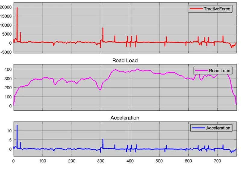
Tractive Force, Road Load and Acceleration :

Post proccesing:

MATLAB coding is used to generate plots a pre written code was given which is named as project1_processingFile which is to be uploaded into thw work space and need to run.

%% Skill-Lync -> Hybrid Drives Development

% Project 1 - Conventional Vehicle Model

% By - Ullekh Gambhira

% Description:

% The following file is to used with the Initialization file and Simulink

% results for post-processing of the data.

% The file is incomplete, has some examples of how the data is imported

% into a readable format, data analysis and plotting examples.

% Based on the project task, use commands in a similar format as given

% below, to analyse the data and generate required plots.

% You can change variable names if desired

%% Post-Processing File

% File for post-processing the Conventional vehicle simulation model data

%% Renaming variables

Time = out.tout;

Acc_Pdl = out.Acc_Pdl; % Accelerator pedal [%]

Brk_Pdl = out.Brk_Pdl; % Brake pedal [%]

Gear_Cmd = out.Gear_Cmd; % Transmission gear

Trans_In_Spd = out.Trans_In_Spd*30/pi; % Transmission input speed [rpm]

Trans_Out_Spd = out.Trans_Out_Spd*30/pi;% Transmission output speed [rpm]

Eng_Trq = out.Eng_Trq; % Engine brake torque [Nm]

Eng_Spd = out.Eng_Spd*30/pi; % Engine speed [rpm]

Eng_Fuel_Consump = out.Eng_Fuel_Consumption; % Engine fuel consumption [g]

Veh_Dist = out.Veh_Dist/1000; % Distance traveled by vehicle [km]

Veh_Spd = out.Veh_Spd*18/5; % Vehicle speed [kmph]

%% Data Analysis

Eng_Pwr = Eng_Spd*pi/30*Eng_Trq/1000; % Engine brake power [kW]

rho_petrol = 0.7197; % Density of petrol [kg/L]

kmpl = Veh_Dist(end)/(Eng_Fuel_Consump(end)/1000/rho_petrol); % Fuel economy [kmpl]

%% Plotting vehicle characteristics time trace

figure()

subplot(3,1,1)

hold on

grid on

plot(Time, Acc_Pdl, 'linewidth', 1, 'Color', 'black');

plot(Time, Brk_Pdl, 'linewidth', 1, 'Color', 'red');

ylabel('Pedal [%]')

xlim([0, Time(end)]);

legend('Accel','Brake');

subplot(3,1,2)

hold on

grid on

plot(Time, Trans_In_Spd, 'linewidth', 1, 'Color', 'black');

plot(Time, Trans_Out_Spd, 'linewidth', 1, 'Color', 'red');

ylabel('Speed [rpm]')

xlim([0, Time(end)]);

ylim([0, 6000]);

legend('Trans Input','Trans Output');

subplot(3,1,3)

hold on

grid on

plot(Time, Gear_Cmd, 'linewidth', 1, 'Color', 'black');

xlim([0, Time(end)]);

xlabel('Time [s]');

ylabel('Gear');

%% Plotting engine operating points on engine fuel map

figure('Name','Engine Operating Points');

hold on

grid on

title('Engine Operating Points','fontsize',12);

p1=plot(Eng_map_spd*30/pi,Eng_max_trq,'linewidth',2,'color','r');

p2=line([Eng_map_spd(end)*30/pi Eng_map_spd(end)*30/pi],[0 Eng_max_trq(end)]);

set(p2,'linewidth',1,'linestyle','--','color','k');

p3=line([Eng_map_spd(1)*30/pi Eng_map_spd(1)*30/pi],[0 Eng_max_trq(1)]);

set(p3,'linewidth',1,'linestyle','--','color','k');

[c,h] = contour(Eng_map_spd'*30/pi,Eng_map_trq,Eng_fuel_map');

clabel(c,h);

xlabel('Engine Speed [rpm]');

ylabel('Engine Torque [Nm]');

title('Engine Fuel Consumption Map [g/s]');

p4 = plot(Eng_Spd,Eng_Trq,'.','color','k');

legend([p1 p4],{'Max Curve','Operating Points'});

axis([Eng_map_spd(1)*30/pi Eng_map_spd(end)*30/pi 0 Eng_map_trq(end)]);

Post processing Plots:

1. Fuel economy numbers (kmpl) for UDDS and HWFET cycle.

UDDS:

HWFET:

As seen from the above data the fuel economy or commonly know as mileage is lower in UDDS than in HWFET because there is less engagement with acceleration pedal in HWFET.

2. The time trace for engine, transmission input, transmission output and wheel speed

UDDS:

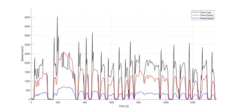
HWFET:

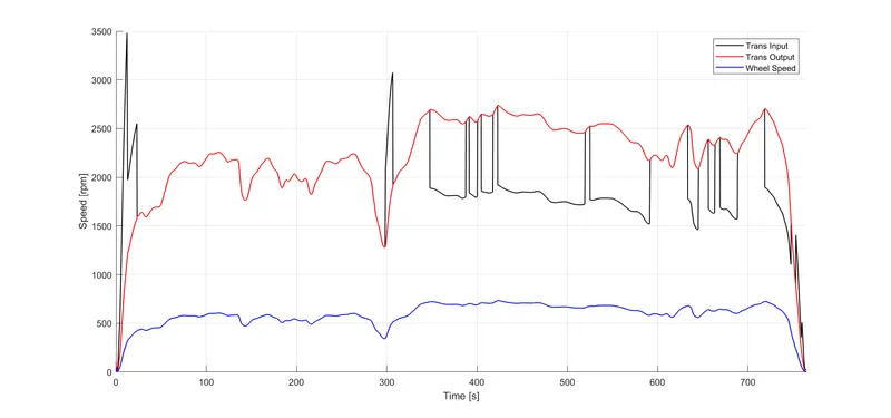
The transmission input speed fluctuates according to the engine torque required in the drive cycle, the Wheel speed and transmission output speed vary according to gear and differential ratio.

3. Engine torque, engine power, fuel rate and fuel consumption

UDDS:

HWFET:

4. Accelerator and brake pedal, gear command, vehicle desired and actual speed, vehicle distance

UDDS:

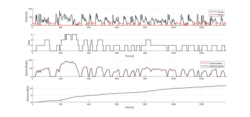
Acceleration and brake pedals are used more because the drive cycle is not very smooth and the gear has to be shifted frequently.

HWFET:

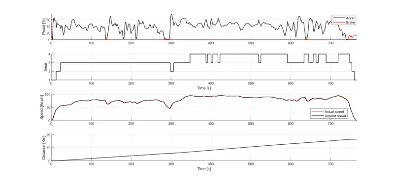
Brake requirements are lower, more accelerator pedals are applied on the highway drive cycle, and gear shifts often occur because the drive cycle is smoother.

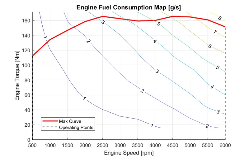
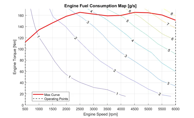
5. The engine operating points on the engine fuel map

UDDS:

HWFET:

Conclusion and results:

The modeling process of a forward energy-based fuel consumption model of a conventional vehicle is designed in MATLAB using codes and simulink in MATLAB.
All the reuired plots during UDDS and HWFET cycle were generated.

Project 1

Ship work like this
in your own course.

Talk to a career counsellor

Ship work like thisin your own course.

Talk to a career counsellor

Ship work like this
in your own course.