Project 2
Description:
As discussed in Lecture 11, Project 2 deals with the development of a forward energy-based fuel consumption model of a P1 hybrid vehicle. This model is based on the conventional vehicle model from Project 1.
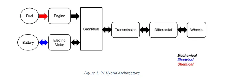
The main goal of this project is to understand the functionality of a P1 hybrid and be able to model it.
Honda Insight motor and battery are considered for this project. Data is taken from ADVISOR data base developed by NREL, USA. Data provided in the project files.

“Project2_InitFile.m” is a Matlab script used to load all the variables required for running the Simulink model and for post-processing. The drive cycle selection is also done here. Before running the Simulink vehicle model, run this initialization script.
Task:
The task of this project is to quantify the improvement in fuel economy numbers for the hybrid vehicle (kmpl), compared to the conventional vehicle, on the urban cycle (UDDS) and highway cycle (HWFET). Also, to analyze and understand the vehicle operating points in terms of engine and motor speed, torque, transmission speeds, pedal positions, gear, distance traveled, battery voltage, current, SoC etc.
To do that, the following steps need to be followed:
1) Load the Project2 folder as the Current Folder in Matlab.
2) Run the “Project2_InitFile.m” Matlab script.
3) Copy the Conventional vehicle Simulink model created for Project 1 in this folder. Figure 1: P1 Hybrid ArchitectureHybrid Drives Development
4) Modify this model into a hybrid vehicle model. The lecture presentations can be used as reference. Battery and Supervisory controller models developed in the assignments can be reused.
5) Add additional ‘To Workspace’ blocks for transferring the desired Simulink vehicle data into the Matlab workspace.
6) Simulate the hybrid model on the desired drive cycles.
7) Write a project report that contains the following:
a. Tabulate the fuel economy numbers (kmpl) for UDDS and HWFET cycle. Compare these numbers with the baseline numbers for conventional vehicle model from Project 1.
b. Plot the time trace for engine, transmission input, transmission output and wheel speed on one plot.
c. Plot engine torque, engine power, fuel rate and fuel consumption using subplots.
d. Plot accelerator and brake pedal, gear command, vehicle desired and actual speed, vehicle distance using subplots.
e. Plot the engine operating points on the engine fuel map.
f. Plot motor speed, torque, motor input power using subplots.
g. Plot pack voltage, current and SoC using subplots.
h. Plot the motor operating points on the motor input power map, with the motor max motoring and generating torque curves.
i. Write down appropriate brief comments on each of these plots, describing the vehicle behavior throughout the drive cycle.
j. Generate the plots for both drive cycles
Ans:
P1 Architecture
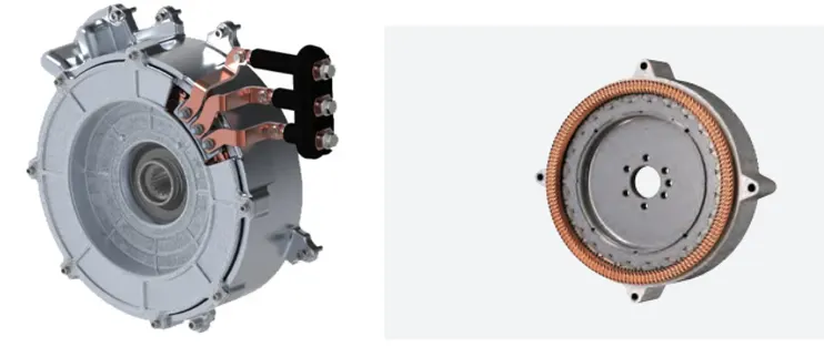
In P1 architecture, Crankshaft-ISG (C-ISG) or Flywheel-Alternator-Starter (FAS), replaces the conventional starter motor and alternator with a larger electric machine located between the engine flywheel and transmission. A P1 architecture typically utilizes conventional transmissions with constructional changes to accommodate electric machine in the same envelope. The electric machine in the P1 architecture may be packaged around torque converter (using a ring type motor) or between the engine and the transmission where the torque converter is removed, such as Honda Integrated-Motor-Assist (IMA) system.
why we use p1 hybrid?
- Adaptable high-performance integrated system for the passenger car, commercial vehicle, and off-highway segments
- Improved system performance and reliability
- Optimized fuel savings and NVH reductions
- More durable and sustainable with reduced CO2 emissions
- Increased powertrain lifetime and enhanced system uptime
- Reduced total cost of ownership
Examples
1)Mclaren P1 hybrid
2) Honda insight Hybrid
Sequence for running the file
1) Initialization file
2) Simulink model
3) post processing file
note: In initialization file set drive cycle select =1 for UDDS and =2 for HWFET
MATLAB PROGRAM
- Initialization script
%% Skill-Lync -> Hybrid Drives Development
% Project 2 - Hybrid vehicle model design
% Description: we are going to design a P1 hybrid

%% Initialization File
% Initialization file for loading the variables for the Conventional vehicle simulation model

%% Vehicle Parameters
M = 1500;       % Vehicle weight [kg]
Cr = 0.015;     % Rolling resistance coefficient
Rw = 0.35;      % Rolling radius [m]
Cd = 0.33;      % Drag coefficient
Af = 2;         % Frontal area [m2]
rhoa = 1.225;   % Air density [kg/m3]
Vwind = 0;      % Wind velocity [kmph]
g = 9.81;       % Gravitational acceleration [m/s2]
theta = 0;      % Slope [deg]
myu_road_tire = 1; % Coefficient of friction between tire - road interface

%% Powertrain Parameters
FDR = 3.73;                         % Final Drive Ratio / Diff Ratio
DiffEff = 0.99;                     % Differential efficiency (assumed independent of operating conditions)

NumGear = 4;                        % Number of gears in transmission
TransGear = [1:NumGear];            % Transmission Gears
TransRatio = [3.06, 1.62, 1, 0.7];  % Corresponding Transmission ratios
TransEff = 0.90;                    % Transmission efficiency (assumed independent of operating conditions)

TC_SR = [0, .5, .6, .7, .8, .87, .92, .94, .96, .97, 1];   % Torque Converter Speed Ratio (Matlab default) -> TurbSpd/PumpSpd
TC_TR = [2.232, 1.5462, 1.4058, 1.2746, 1.1528, 1.0732, 1.0192, 1, 1, 1, 1];   % Torque Converter Torque Ratio (Matlab default) -> TurbTrq/PumpTrq
TC_Cf = 1e-4 * [.72558, .66322, .63463, .59042, .51331, .4144, .29287, .22444, .12186, .04386, 0]; % Torque Converter Capacity Factor (Matlab default) -> PumpTrq/PumpSpd^2 [Nm/rpm^2]

load Vehicle_Data/Engine_data_1_9L_Saturn_95kW
load Vehicle_Data/Trans_Shift_map
load Vehicle_Data/EM_Honda_Insight_10kW
load Vehicle_Data/ESS_NiMH6


ESS_init_soc = 0.8;
ESS_soc_max = 0.9;
ESS_soc_min = 0.6;


%% Driver Parameters
Kp = 10;                    % P gain for driver PI model
Ki = 1;                     % I gain for driver PI model
Drive_Cycle_Select = ;
% Drive cycle selection

% Drive cycle values in m/s

if Drive_Cycle_Select == 1
    load DriveCycles/UDDS;

elseif Drive_Cycle_Select == 2
    load DriveCycles/HWFET;

elseif Drive_Cycle_Select == 3
    load DriveCycles/FTP;

elseif Drive_Cycle_Select == 4
    load DriveCycles/US06;

elseif Drive_Cycle_Select == 5
    load DriveCycles/NEDC;

elseif Drive_Cycle_Select == 6
    load DriveCycles/WLTP;

end

time_end = cyc_time(end);
vel_end = cyc_vel(end);- Post processing script
%%%%%%%%%%%%%%%%%%%%%%%%%%%%%%%%%%%%%%%%%%%%%%%%%%%%%%%%%%%%%%%%%%%%%
%% Skill-Lync -> Hybrid Drives Development
% Project 2 - Hybrid vehicle model
%

% Description:
% we have extracted all the desired values from simulink model and plotted
% the graph to obtain the characteristics of our P1 hybrid

%% Post-Processing File
%  File for post-processing the Conventional vehicle simulation model data

%% Renaming variables
Time = out.tout;
Acc_Pdl = out.Acc_Pdl;          % Accelerator pedal [%]
Brk_Pdl = out.Brk_Pdl;          % Brake pedal [%]
Gear_Cmd = out.Gear_Cmd;        % Transmission gear
Trans_In_Spd = out.Trans_In_Spd*30/pi;  % Transmission input speed [rpm]
Trans_Out_Spd = out.Trans_Out_Spd*30/pi;% Transmission output speed [rpm]
Eng_Trq = out.Eng_Trq;          % Engine brake torque [Nm]
Eng_Spd = out.Eng_Spd*30/pi;    % Engine speed [rpm]
Eng_Fuel_Consump = out.Eng_Fuel_Consumption;    % Engine fuel consumption [g]
Veh_Dist = out.Veh_Dist/1000;   % Distance traveled by vehicle [km]
Veh_Spd = out.Veh_Spd*18/5;     % Vehicle speed [kmph]


%% Data Analysis
Eng_Pwr = Eng_Spd.*pi/30.*Eng_Trq/1000;   % Engine brake power [kW]
rho_petrol = 0.7197;                    % Density of petrol [kg/L]
kmpl = Veh_Dist(end)/(Eng_Fuel_Consump(end)/1000/rho_petrol);    % Fuel economy [kmpl]


%% Plotting vehicle characteristics time trace
figure(1)
subplot(3,1,1)
hold on
grid on
plot(Time, Acc_Pdl, 'linewidth', 1, 'Color', 'black');
plot(Time, Brk_Pdl, 'linewidth', 1, 'Color', 'red');
ylabel('Pedal [%]')
xlim([0, Time(end)]);
legend('Accel','Brake');
subplot(3,1,2)
hold on
grid on
plot(Time, Trans_In_Spd, 'linewidth', 1, 'Color', 'black');
plot(Time, Trans_Out_Spd, 'linewidth', 1, 'Color', 'red');
ylabel('Speed [rpm]')
xlim([0, Time(end)]);
ylim([0, 6000]);
legend('Trans Input','Trans Output');
subplot(3,1,3)
hold on
grid on
plot(Time, Gear_Cmd, 'linewidth', 1, 'Color', 'black');
xlim([0, Time(end)]);
xlabel('Time [s]');
ylabel('Gear');

%% Plotting engine operating points on engine fuel map
figure(2);
hold on
grid on
title('Engine Operating Points','fontsize',12);
p1=plot(Eng_map_spd*30/pi,Eng_max_trq,'linewidth',2,'color','r');
p2=line([Eng_map_spd(end)*30/pi Eng_map_spd(end)*30/pi],[0 Eng_max_trq(end)]);
set(p2,'linewidth',1,'linestyle','--','color','k');
p3=line([Eng_map_spd(1)*30/pi Eng_map_spd(1)*30/pi],[0 Eng_max_trq(1)]);
set(p3,'linewidth',1,'linestyle','--','color','k');
[c,h] = contour(Eng_map_spd'*30/pi,Eng_map_trq,Eng_fuel_map');
clabel(c,h);
xlabel('Engine Speed [rpm]');
ylabel('Engine Torque [Nm]');
title('Engine Fuel Consumption Map [g/s]');
p4 = plot(Eng_Spd,Eng_Trq,'.','color','k');
legend([p1 p4],{'Max Curve','Operating Points'});
axis([Eng_map_spd(1)*30/pi Eng_map_spd(end)*30/pi 0 Eng_map_trq(end)]);

 figure(3)
hold on
grid on
 subplot(3,1,1)
 plot(Time,out.Eng_Spd,'linewidth', 1, 'Color','g')
  title('Engine speed characteristics')
 xlabel('Time')
 ylabel('Engine speed')
  subplot(3,1,2)
plot(Time,out.Eng_Trq,'linewidth', 1, 'Color','c')
  title('Engine torque characteristics')
xlabel('Time')
 ylabel('Engine torque')
    subplot(3,1,3)
   plot(Time,out.Eng_Fuel_Consumption, 'linewidth', 1, 'Color','k')
     title('Engine fuel consumption characteristics')
   xlabel('Time')
 ylabel('Engine fuel consumption')

 figure(4)
 hold on
grid on
 subplot(3,1,1)
plot(Time,out.EM_speed,'linewidth', 1, 'Color','m')
title('Electric motor speed characteristics')
 xlabel('Time')
 ylabel('Electric motor speed')
  subplot(3,1,2)
  plot(Time,out.EM_power,'linewidth', 1, 'Color','c')
  title('Electric motor power characteristics')
 xlabel('Time')
 ylabel('Electric motor power')
subplot(3,1,3)
  plot(Time,out.EM_torque,'linewidth', 1, 'Color','r')
  title('Electric motor torque characteristics')
 xlabel('Time')
 ylabel('Electric motor torque')

 figure(5)
 hold on
grid on
 subplot(3,1,1)
plot(Time,out.SOC,'linewidth', 1, 'Color','c')
title('Battery pack SOC  characteristics')
 xlabel('Time')
 ylabel('State of charge')
 subplot(3,1,2)
plot(Time,out.terminal_voltage,'linewidth', 1, 'Color','k')
title('Battery pack Terminal voltage characteristics')
 xlabel('Time')
 ylabel('Terminal voltage')
 subplot(3,1,3)
plot(Time,out.current,'linewidth', 1, 'Color','b')
title('Battery pack  current characteristics')
 xlabel('Time')
 ylabel('Current')

 figure(6)
 hold on
grid on
 subplot(2,1,1)
plot(Time,out.Veh_Dist,'linewidth', 1, 'Color','r')
 title('Distance covered')
 xlabel('Time')
 ylabel('distance')
 subplot(2,1,2)
 plot(Time,out.Veh_Spd,'linewidth', 1, 'Color','g')
 title('Vehicle speed  characteristics')
 xlabel('Time')
 ylabel('speed')
SIMULINK MODELS
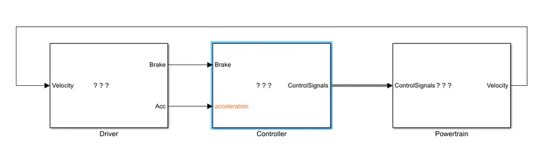
note: Additional modifications made to the block are highlited with orange color
1)DRIVER BLOCK
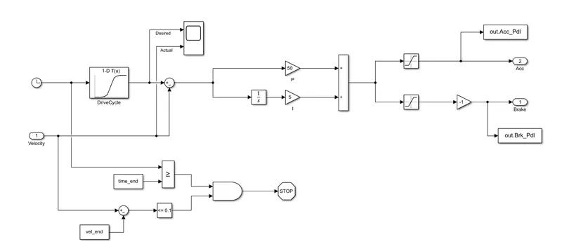
Driver block consists of a PI controller which is used to match acceleration and braking actual output with desired output
2) CONTROLLER BLOCK
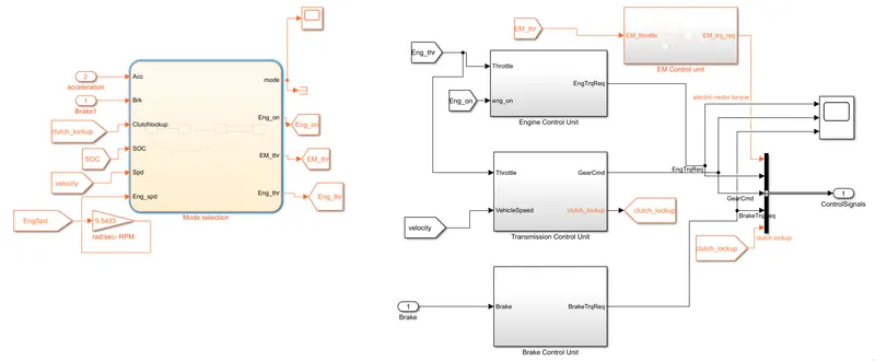
Controller consists of mode selection chart which takes in input values. Checks for the conditions inside the chart and gives desired output. Then there is additional control unit for Engine, transmission, brake and electric motot.
- A)ENGINE CONTROL UNIT
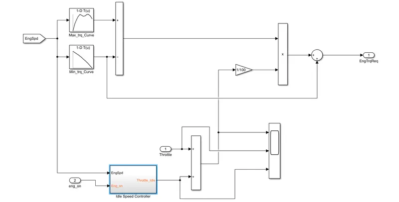
This model controls engine speed, throttle and engine on off condition. The torque is limited between a certain minimum and maximum range. Here the engine speed, engine-on and throttle are the inputs and the output is engine torque requirment
- A) 1) IDLE SPEED CONTROLLER
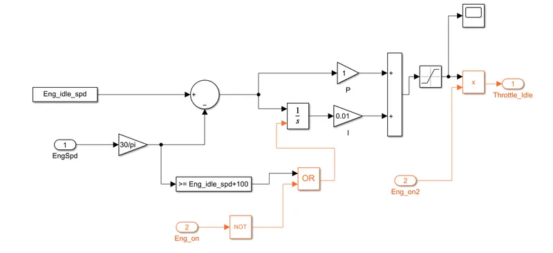
this Block decides when to turn on and off the engine with the help of logic operation
- B)TRANSMISSION CONTROL UNIT
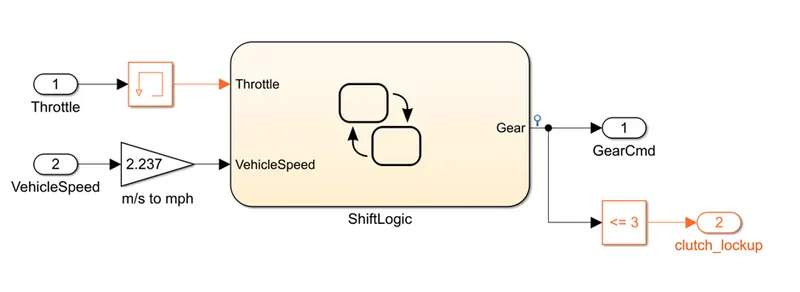
it is not easy to lockup the clutch in small gears because At low speeds we don’t have much pressure and ot of torque multiplication in lower gears so this will be felt by driver. so we are locking up the clutch when the gear is above 3rd
- C) ELECTRIC MOTOR CONTROL UNIT
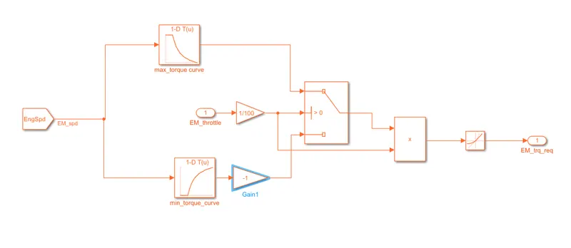
Here we input the speed and throttle to obtrain the torque requirment in the output.
3) POWER TRAIN BLOCK
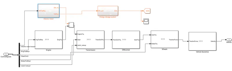
Since we are developing a hybrid we have added an electric motor and energy storage system.
- A) ELECTRIC MOTOR
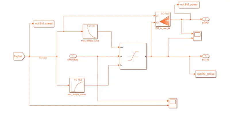
This block takes engine speed as input, these speeds are provided to maps. A saturation block is used to output the torque such that the Electric motor torque value is maintained between minimum and maximum torque and also electric motor power is obtained.
- B) ENGINE
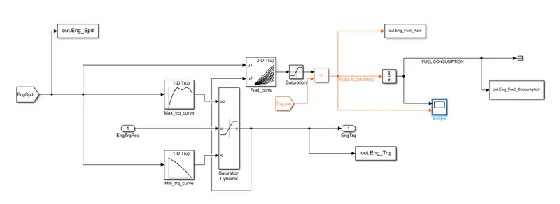
The engine consists of speed input, the torque is saturated between max and min torque. The fuel flow rate and fuel consumption is computed here.
- C) ENERGY STORAGE SYSTEM
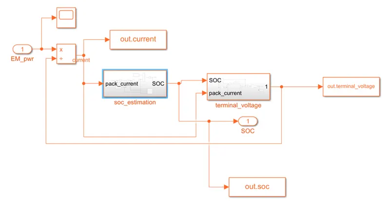
Here Power is the input and it divided by voltage to get current so we get treminal voltage and current. SOC is also determined here
A) UDDS CYCLE
PLOT 1
- time trace for engine, Acceleration and braking (subplot-1)
- time trace for engine, transmission input, transmission output and wheel speed (subplot-2)
- Time VS gear command (subplot-3)
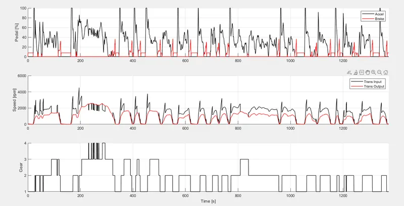
here we can see the acceleration and braking happening, transmission input and output speed and also the gear change during this duration for UDDS Cycle
PLOT 2
- Fuel consumption map (with engine torque, speed, fuel rate and consumption)
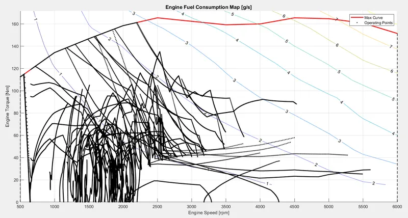
here we can see the engine speed and torque at different operating points and the max curve region for UDDDS Cycle
PLOT 3
- Engine speed VS time (subplot-1)
- Engine torque VS time (subplot-2)
- Engine fuel consumption VS time (subplot-3)
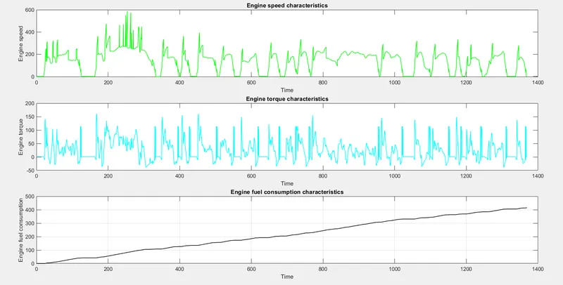
Here since there is a lot of stop and start condition we can see there is a sudden increase and decrease in speed and torque and the fuel consumption after the cycle can also be seen
PLOT 4
- Electric motor speed VS time (subplot-1)
- Electric motor power VS time (subplot-2)
- Electric motor torque VS time (subplot-3)
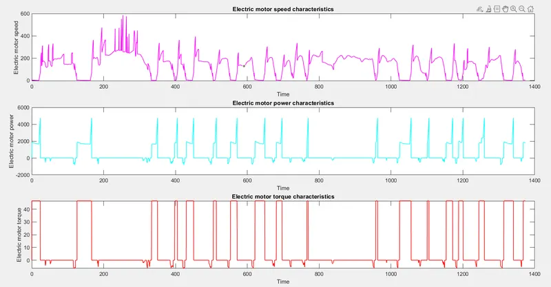
Just like we previously said since there is a lot of start and stop condition we can see sudden incerase and decrease in Electric motor speed and torque.
PLOT 5
- Battery pack SOC VS time (subplot-1)
- Battery pack Terminal voltage VS time (subplot-2)
- Battery pack current VS time (subplot-3)
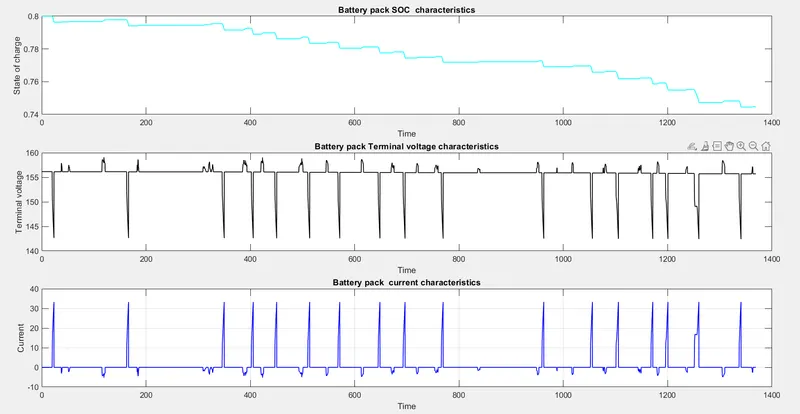
We can see that we have set the initial SOC to be 80% and after the cycle the charge gets depleted to below 75%. As per the power requirments the battery pack current and voltage will vary
PLOT 6
- Distance covered VS time (subplot-1)
- vehicle speed VS time (subplot-2)
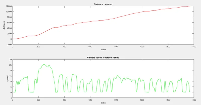
we can see that the vehicle model covered a max of 12000m with with speed varying from 0-25KMPH for UDDS cycle
Fuel efficency obtained
B) HWFET CYCLE
PLOT 1
- time trace for engine, Acceleration and braking (subplot-1)
- time trace for engine, transmission input, transmission output and wheel speed (subplot-2)
- Time VS gear command (subplot-3)
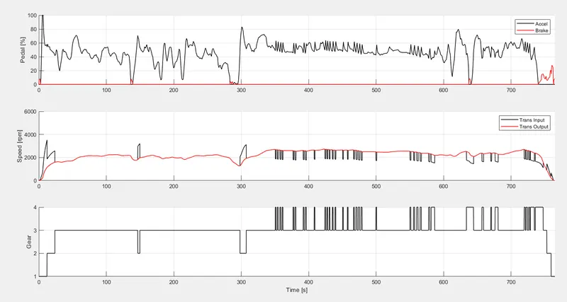
here we can see the acceleration and braking happening, transmission input and output speed and also the gear change during this duration for UDDS Cycle
PLOT 2
- Fuel consumption map (with engine torque, speed, fuel rate and consumption)
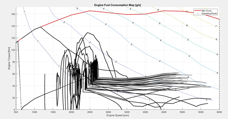
here we can see the acceleration and braking happening, transmission input and output speed and also the gear change during this duration for HWFET Cycle
PLOT 3
- Engine speed VS time (subplot-1)
- Engine torque VS time (subplot-2)
- Engine fuel consumption VS time (subplot-3)
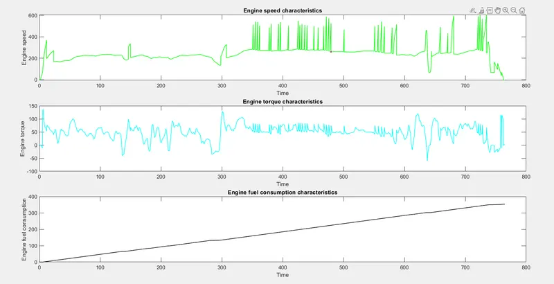
We can see the Speed torque and fuel consumption for HWFET cycle. Here it is a highway driving condition so there is less braking and more constant speed which can be observed in the graph. The fuel consumption after the cycle can also be seen
PLOT 4
- Electric motor speed VS time (subplot-1)
- Electric motor power VS time (subplot-2)
- Electric motor torque VS time (subplot-3)
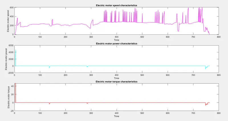
Since this is a highway condtiton there is sudden increase and decrease of speed
PLOT 5
- Battery pack SOC VS time (subplot-1)
- Battery pack Terminal voltage VS time (subplot-2)
- Battery pack current VS time (subplot-3)
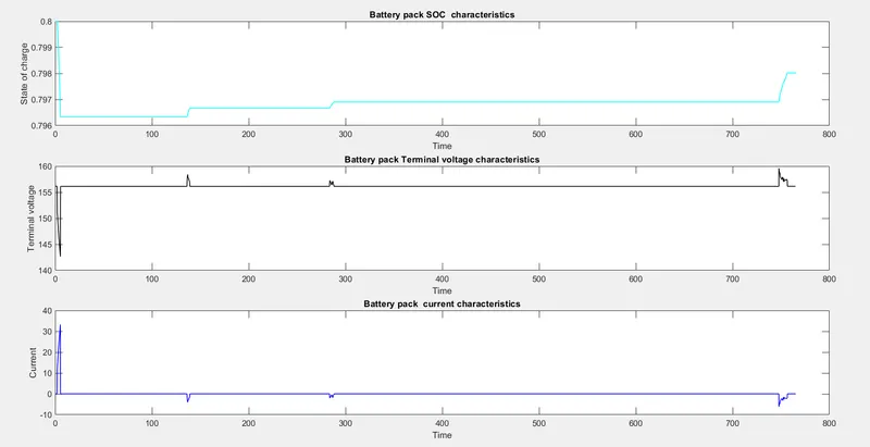
We can see that we have set the initial SOC to be 80% and after the cycle the charge gets depleted a bit. since we have a small depletion in SOC so the graph is in expanded view so we can see the battey SOC rises, this is due to the battery getting charged by regenerative braking. As per the power requirments the battery pack current and voltage will vary.
PLOT 6
- Distance covered VS time (subplot-1)
- vehicle speed VS time (subplot-2)
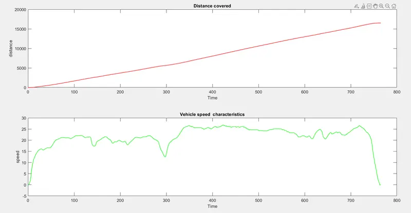
we can see that the vehicle model covered a max of 15000m with with almost constant sped since it is is HWFET consist of highway driving condition so there is no start stop.
FUEL CONSUMPTION COMPARISON
- EARLIER: IC ENGINE
UDDS:11.39KMPL
HWFET:15.459 KMPL
- NOW: HYBRID
UDDS: 20.8 KMPL
HWFET: 33.64 KMPL
By the addition of P1 hybrid we have seen that our fuel efficency has risen drastically.