Project 2

AIM: The main goal of this project is to understand the functionality of a P1 hybrid and be able to model it.

PROCEDURE:

1) Load the Project2 folder as the Current Folder in Matlab.
2) Run the “Project2_InitFile.m” Matlab script.

The script is mentioned below:

% Project 2 - Hybrid Vehicle Model
% By - Ullekh Gambhira 

% Description:

%% Initialization File
% Initialization file for loading the variables for the Conventional vehicle simulation model

%% Vehicle Parameters
M = 1500;       % Vehicle weight [kg]
Cr = 0.015;     % Rolling resistance coefficient
Rw = 0.35;      % Rolling radius [m]
Cd = 0.33;      % Drag coefficient
Af = 2;         % Frontal area [m2]
rhoa = 1.225;   % Air density [kg/m3]
Vwind = 0;      % Wind velocity [kmph]
g = 9.81;       % Gravitational acceleration [m/s2]
theta = 0;      % Slope [deg]
myu_road_tire = 1; % Coefficient of friction between tire - road interface

%% Powertrain Parameters 
FDR = 3.73;                         % Final Drive Ratio / Diff Ratio
DiffEff = 0.99;                     % Differential efficiency (assumed independent of operating conditions)

NumGear = 4;                        % Number of gears in transmission
TransGear = [1:NumGear];            % Transmission Gears
TransRatio = [3.06, 1.62, 1, 0.7];  % Corresponding Transmission ratios
TransEff = 0.90;                    % Transmission efficiency (assumed independent of operating conditions)

TC_SR = [0, .5, .6, .7, .8, .87, .92, .94, .96, .97, 1];   % Torque Converter Speed Ratio (Matlab default) -> TurbSpd/PumpSpd  
TC_TR = [2.232, 1.5462, 1.4058, 1.2746, 1.1528, 1.0732, 1.0192, 1, 1, 1, 1];   % Torque Converter Torque Ratio (Matlab default) -> TurbTrq/PumpTrq
TC_Cf = 1e-4 * [.72558, .66322, .63463, .59042, .51331, .4144, .29287, .22444, .12186, .04386, 0]; % Torque Converter Capacity Factor (Matlab default) -> PumpTrq/PumpSpd^2 [Nm/rpm^2]

load Vehicle_Data/Engine_data_1_9L_Saturn_95kW
load Vehicle_Data/Trans_Shift_map
load Vehicle_Data/EM_Honda_Insight_10kW
load Vehicle_Data/ESS_NiMH6


ESS_init_soc = 0.8;
ESS_soc_max = 0.9;
ESS_soc_min = 0.6;


%% Driver Parameters
Kp = 10;                    % P gain for driver PI model
Ki = 1;                     % I gain for driver PI model
Drive_Cycle_Select = 2;     % Drive cycle selection

% Drive cycle values in m/s

if Drive_Cycle_Select == 1
    load DriveCycles/UDDS;
    
elseif Drive_Cycle_Select == 2
    load DriveCycles/HWFET;
    
elseif Drive_Cycle_Select == 3
    load DriveCycles/FTP;
    
elseif Drive_Cycle_Select == 4
    load DriveCycles/US06;
    
elseif Drive_Cycle_Select == 5
    load DriveCycles/NEDC;
    
elseif Drive_Cycle_Select == 6
    load DriveCycles/WLTP;
 
end

time_end = cyc_time(end);
vel_end = cyc_vel(end);

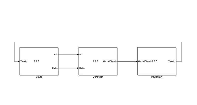
3) Copy the Conventional vehicle Simulink model created for Project 1 in this folder. Figure 1: P1 Hybrid ArchitectureHybrid Drives Development

The model is given below:

4) Modify this model into a hybrid vehicle model.

5) Add additional ‘To Workspace’ blocks for transferring the desired Simulink vehicle data into the Matlab workspace.

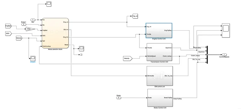
After analysing the conventional vehicle model suitable changes has been done in the following blocks:

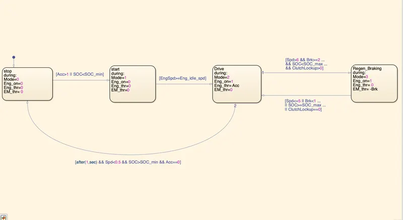
a. In the controller we added a supervisory controller which is the mode selection block. It selects which mode the vehicle is running.

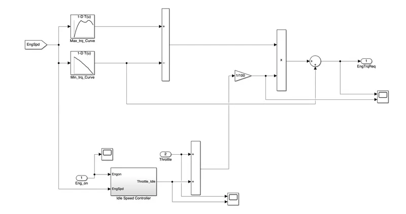
b. In engine control unit we added an engine ON/OFF functionality to turn off the idle speed controller when the vehicle is in off condition, so that no torque request is given.

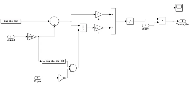
c. In transmission control unit addition of clutch lockup is done.

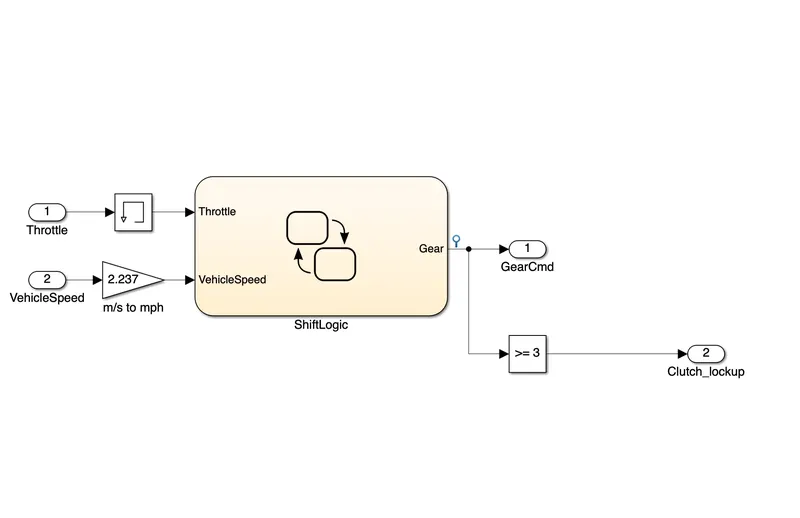
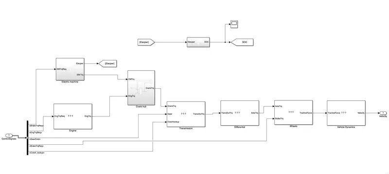
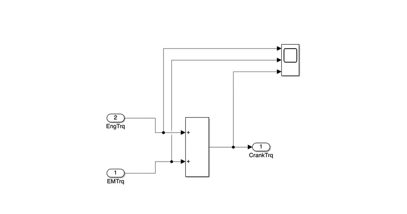
d. In power train block the engine and electric motor are connected to crankhub and both of the torque will add up provide crank torque. Also, a battery is provided as a stand alone unit which provide electrical supply to accesories.

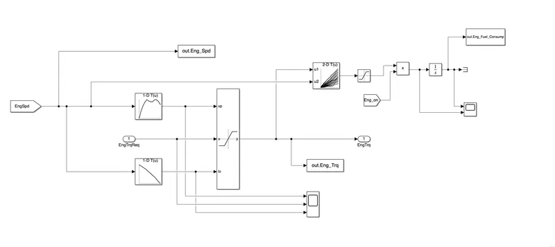
e. In engine, multiplying the engine ON value with the fuel consumption to force the fuel consumption to zero when the engine is in OFF condition.

f. To model an electric motor.

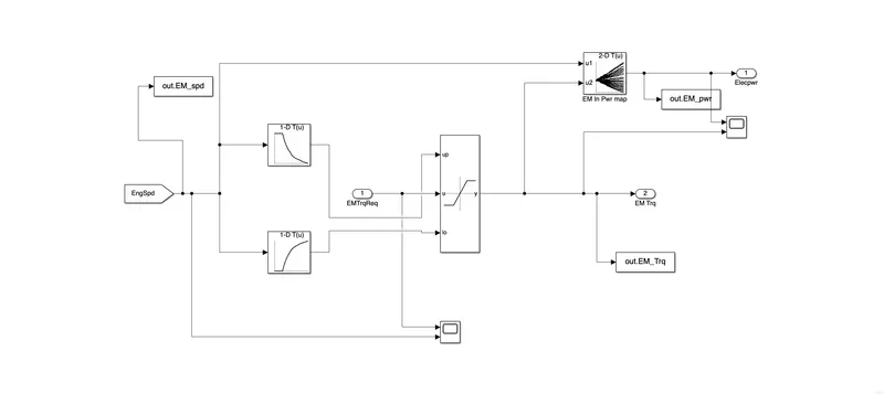
g. Providing a crank hub in the power train block which add up the engine torque and EM torque.

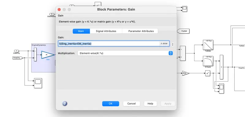
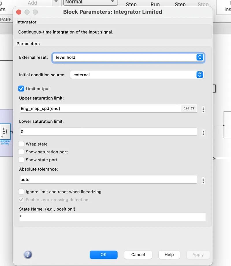
h. In transmission, changes done is on the vehicle dynamics of torque converter block by adding EM inertia along with Engine inertia. Also couple of changes done in the integrator block.

i. Adding of clutch lockup to lock up the pump speed and the turbine speed, also when the clutch open the pump speed and the turbine speed will be different which will lead to speed ratios.

j. Adding a switch block to decide the input torque to the transmission i.e., if the clutch lock up is zero then turbine torque will be selected and when the clutch is locked up then transmission input torque is the crank torque.

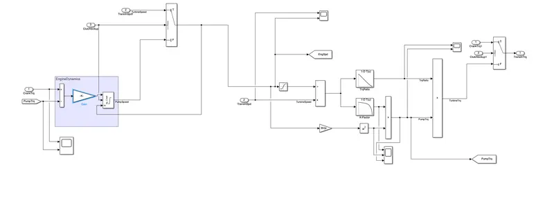
Tabulate the fuel economy numbers (kmpl) for UDDS and HWFET cycle. Compare these numbers with the baseline numbers for conventional vehicle model from Project 1:

	UDDS	HWFET
conventional vehicles (kmpl)	13.6	16.3
Hybrid electric vehicles (kmpl)	15.14	16.998

As from the values we can conclude that Hybrid electric vehicles are more energy efficient than conventional vehicle and if we run the motor for prolonged period we will get more improved values

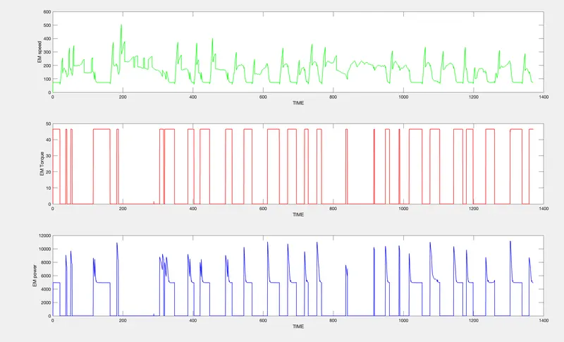
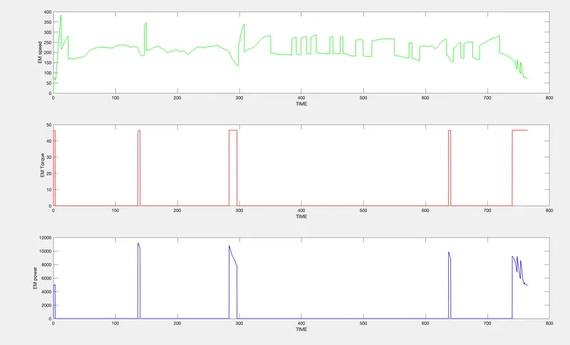
Plot motor speed, torque, motor input power using subplots.

UDDS

HWFET:

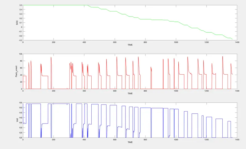
Plot the motor operating points on the motor input power map, with the motor max motoring and generating torque curves.

UDDS

HWFET

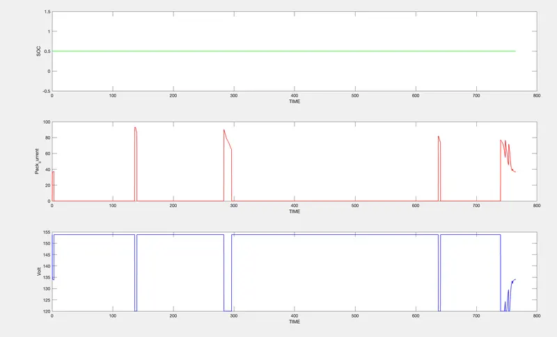
MOTOR OPERATING POINTS

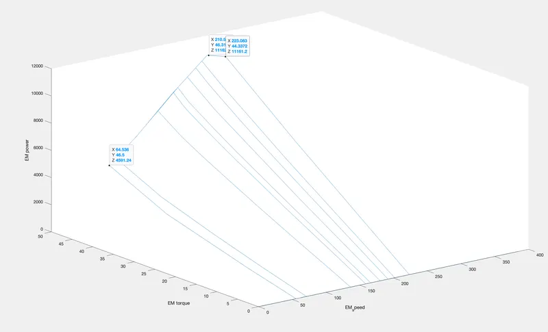
From the plots we can conclude that HWFET is using less motor due to highway running but UDDS cycle the use of the motor is in considerable amount due to which it is evident that hybrid electric vehicle will have considerable amount of energy savings in UDDS cycle than HWFET.