Project 2

AIM

DEVELOPMENT OF A FORWARD-BASED FUEL CONSUMPTION OF A HYBRID VEHICLE

OBJECTIVES

• To find the fuel economy of UDDS and HWFET cycle. We will compare it with conventional vehicle.
• Plot the time trace for engine, transmission input, transmission output and wheel speed on one plot
• With the help of subplots plot engine torque, engine power, fuel rate and fuel consumption.
• with the help of subplots Plot accelerator and brake pedal, gear command, vehicle desired and actual speed, vehicle distance.
• With the help of subplots Plot motor speed, torque, motor input power.
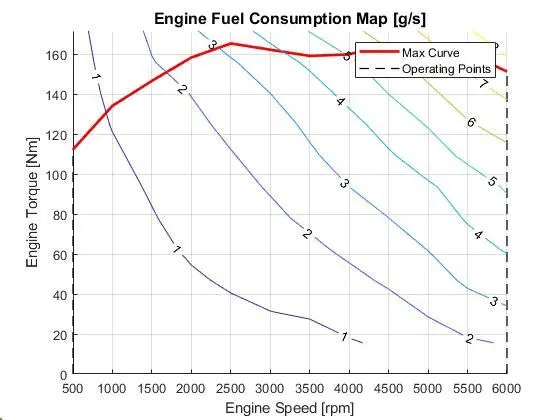
• Plot the engine operating points on the engine fuel map.
• Using subplots plot pack voltage, current and SOC.
• Plot the motor operating points on the motor input power map, with the motor max motoring and generating torque curves.
• We will generate the plots for UDDS and HWFET cycle.

THEORY

P1 Mild Hybrid Electric Vehicle

Honda chose the P1 architecture for their first-generation Integrated Motor Assist (IMA) technology because it allows the electric motor to be connected directly to the crankshaft. The electric motor serves as a generator, an engine starter, a motor (to help the engine), and a generator during vehicle braking. The fact that the electric motor can deliver more torque than the BiSG because there is no belt restriction is one of the solution's main benefits (due to slip). The torque demands on the electric motor, however, can be fairly high because there is no speed to torque relationship between the electric machine and crankshaft.

Two examples of P1 MHEV architectures are:

• Honda Insight Hybrid 2009 (with Integrated Motor Assist technology)
• Mercedes Benz S400 Bluehybrid 2010

For example, the main characteristics of the P1 MHEV.

1] ELectric Machine Performance

Maximum torque up to 34 Nm.

Maximum power: 10KW

Efficiency: Up to 94 Percent.

2] Hybrid Modes

Idle stop and stop

Moving stop and start

Engine load shift

Torque assist

Torque boost

Energy recuperation

Brake generation

3] Advantages

Higher efficiency

The 12V starter can be removed.

4] Disadvantages

The torque is limited by size of the motors.

Energy recuperation affected by engine friction losses

High impact on existing vehicle architecture

Higher overall cost of the electrical components

Air cooling not possible for electric machine

5] Overall characteristics

Toruqe Boosting capacity: High

Electrical energy recuperation: Medium

Driveability improvements: Medium

Electrical Creep/drive: Possible

MODEL DESCRIPTION

It is often referred to as dynamic modelling. In-depth simulations are performed using dynamic models. This model uses force, torque, and power as inputs and vehicle status variables, such as acceleration and velocity, as outputs. Due to physical casualty, models and simulations are more realistic and suitable for control development. To achieve the desired vehicle state, there is a feedback loop. It is primarily used to replicate a vehicle while it is being driven in order to analyse the dynamic behavior of the system, which greatly aids in the creation of controls.

PROCESS

Load the Project2 folder as the Current Folder in Matlab.

Run the “Project2_InitFile.m” Matlab script.

The Drive cycle selection is done here.

MATLAB CODE

After run this coding file open simulink model.

BLOCK DIAGRAMS

BLOCK DIAGRAM OF DRIVER CONTROLLER AND VEHICLE PLANT

SIMULINK MODEL FOR POWERTRAIN UNIT

SIMULINK MODEL FOR DRIVER UNIT

A "Driver" block, a fundamental PI controller, is used to model it. It creates outputs for the accelerator and brake pedals that correspond to the desired and actual vehicle speeds. We use drive cycles for this since they serve as a basis for uniform assessment and the outcomes of fuel consumption and emissions certification for the vehicle. It is based on time and velocity, after which everything is integrated to produce the accelerator and brake pedals.

SIMULINK MODEL FOR CONTROLLER UNIT

The controller block, which stands in for the electronic control systems, is the brains of the car. It produces the required engine torque, desired transmission gear, desired motor torque, and desired brake torque dependent on the driver's inputs. These inputs are supplied to the "Powertrain" block, which symbolises the car's drivetrain. This calls for the creation of a stateflow block, as seen in the following diagram.

STATEFLOW FOR CONTROLLER

The four circumstances we created in this were stop, start, drive, and regenration braking. The halt condition is represented by the first block. wherein the engine is turned off. There is no throttle applied to the engine or the motor. The second block represents the commencement condition after that. When the electric motor is in mode 1, the throttle is solely used to give the car the necessary torque and power. Engine throttle condition is zero and the engine is not running.

The linkages connect states 1 and 2, so when acceleration is less than one or SOC is less than the minimum SOC, it switches between states 1 and 2.

State 3 represents mode 2, meaning that the engine is running and that the driver has applied a positive value to the engine throttle, but that the electric motor throttle is at zero. When the engine speed is greater than or equal to the engine idle speed, it transitions from state 2 to state 3.

Model 3's regenrative braking is represented by state 4, The engine is running in this situation, but the driver is not controlling the engine throttle, while the electric motor receives negative power from braking.

Acceleration, barke, engine speed, vehicle speed, SOC, and clutch lockup are the inputs for the chart.

Mode, engine condition, engine throttle condition, and electric motor throttle condition are the outputs we get from the chart.

Modification done in all Unit modeling. they showed in next figures.

SIMULINK MODEL FOR ENGINE CONTROL UNIT

We use an engine control unit in this control model, which provides input for the engine speed by building a look-up table. We feed Maximum torque and map speed into that table, and we also establish a second look-up table in which we input CT torque and map speed, from which it subtracts and multiplies. The engine speed also provides the correct counterspeed to integrate, and as a result, the engine's required torque output is met.

SIMULINK MODEL FOR TRANSMISSION CONTROL UNIT

In this unit we create steadfy flow variable state for controlling of gears of vehicle as in ascending and descending order with respect to time, speed, distance. and give input to this steady state is vehicle speed in m/s to mph.

SHIFT LOGIC UNIT

IDLE SPEED IN CONTROLLER

SIMULINK MODEL FOR ELECTRIC MOTOR CONTROL UNIT

Motor controllers are devices that regulate the operation of an electric motor. In artificial lift applications, motor controllers generally refer to those devices used in conjunction with switchgear or variable frequency drives to control prime mover operation.

SIMULINK MODEL FOR BRAKE CONTROL UNIT

SIMULINK MODEL FOR ENGINE UNIT

To model the engine's fuel consumption in this model, we employed a map-based model. It is based on the controller's maximum torque and minimum torque. and then it takes the speed and torque, goes into saturated output, and then gives the output before saturated torque and speed map produce fuel consumption.

SIMULINK MODEL FOR ELECTRIC MOTOR UNIT

An electric motor is an electrical machine that converts electrical energy into mechanical energy. Most electric motors work through the interaction between the motor's magnetic field and the electric current in the wire winding to create force in the form of torque applied to the motor shaft.

SIMULINK MODEL FOR CRANK HUB UNIT

The Stock Crank Hub design allows the pinion to rotate independently of the cranks, causing the user to re-time the engine to a minimum, and in the worst case scenario, piston-to-valve contact will damage the engine and require a complete engine overhaul.

SIMULINK MODEL FOR TRANSMISSION UNIT

In these models, we use the gear selector from the controllerb for transmission of the gear ratio and the engine torque. The gearbox input speed is determined by multiplying the ratio by the transmission input torque, positive torque, and negative torque, respectively. In this instance, the torque converter is a transmission component that connects the engine to the transmission. It essentially has decoupled engine dynamics.

SIMULINK MODEL FOR TORQUE CONVERTER UNIT

SIMULINK MODEL FOR DIFFERENTIAL UNIT

Axle torque is then met after the transmission's output has been multiplied by the input and output torques and passed through the differential ratio. The differential ratio and transmission torque are greater than the axle torque.

SIMULINK MODEL FOR WHEEL UNIT

In this model, we take the braking torque from the controller and the axle torque from the differential. Rolling radius and speed are subtracted from and multiplied before we encounter the tractive force from axle and braking torque. and velocity is used to satisfy the wheelspeed.

SIMULINK MODEL FOR VEHICLE DYNAMICS

BATTERY MANAGEMENT

SIMULINK MODEL FOR ESTIMATED STORAGE SYSTEM

We provide input as power, which is multiplied and converted to output as pack current. After that, the terminal voltage is given as input and is then met as the output of the soc estimation meet output SOC.

SIMULINK MODEL FOR TERMINAL VOLTAGE

The first table variable in this use input SOC is interpolated as the state of charge and the open voltage circuit. It is coupled to a 1D lookup table. Resistance discharge and state of charge were interpolated as variables in the second table, and resistance charge and state of charge were interpolated as variables in the third table. The switch block is then given control over the three-shold. then they provide maximum and minimum voltage restrictions. meet terminal voltage after that.

SIMULINK MODEL FOR SOC ESTIMATION

A battery's SOC, i.e. its remaining capacity, can be determined using a discharge test under controlled conditions. The voltage method converts the battery voltage reading to an equivalent SOC value using the known discharge curve (voltage vs. SOC) of the battery.

SIMULINK MODEL FOR PACK CURRENT

In this we integrate pack current and convert it rad to amp then saturated and meet SOC.

Then we create one coding file for creating plots and to meet all answers. that file shown in next.

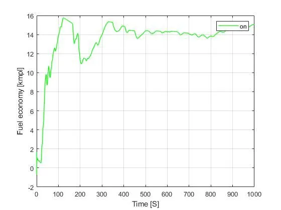
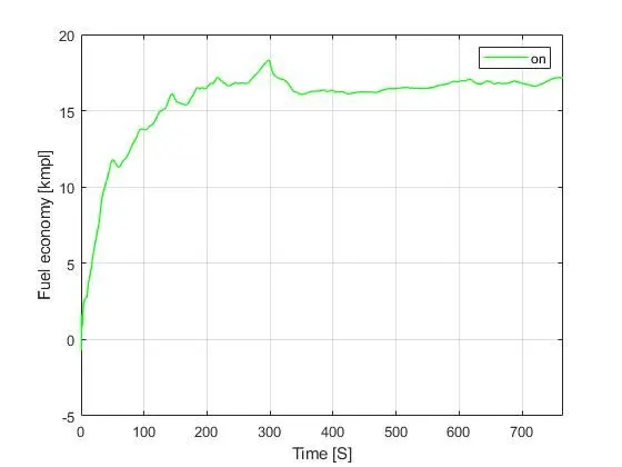
a. Tabulate the fuel economy numbers (kmpl) for UDDS and HWFET cycle. Compare these numbers with the baseline numbers for conventional vehicle model from Project 1.

As can be seen, HWFET has higher fuel efficiency than UDDS. This is due to the fact that when driving in cities, there is more traffic, stops are required more frequently, and gasoline consumption is higher at first. Because there is no traffic and the car is moving without excessive braking during HWFET, the fuel economy rating is higher.

When we can see, project 2's fuel economy figures are a little higher than project 1's because it has an electric motor installed. Because project 2 is a P1 hybrid, the fuel economy may not vary much, but as we add additional architectural features, it will rise dramatically.

b) Plot the time trace for engine, transmission input, transmission output and wheel speed on one plot

UDDS CYCLE

MATLAB CODE

%Plot the time trace for engine, transmission input, transmission output and wheel speed on one plot.

% plot for UDDS CYCLE

figure(1)

hold on

grid on

plot(out.tout,out.Trans_In_Spd,'LineWidth',1,'Color','red');

plot(out.tout,out.Trans_Out_Spd,'LineWidth',1,'Color','black');

plot(out.tout,out.wheelspd,'LineWidth',1,'Color','blue');

xlabel('Time(s)');

ylabel('Speed(rpm)');

xlim([0,1000]);

ylim([0,1000]);

ylim([0,500]);

legend('Trans input','Trans out','Wheel speed');

HWFET CYCLE

MATLAB CODE

%Plot the time trace for engine, transmission input, transmission output and wheel speed on one plot.

% plot for HWFET CYCLE

figure(1)

hold on

grid on

plot(out.tout,out.Trans_In_Spd,'LineWidth',1,'Color','red');

plot(out.tout,out.Trans_Out_Spd,'LineWidth',1,'Color','black');

plot(out.tout,out.wheelspd,'LineWidth',1,'Color','blue');

xlabel('Time(s)');

ylabel('Speed(rpm)');

xlim([0,1000]);

ylim([0,1000]);

ylim([0,500]);

legend('Trans input','Trans out','Wheel speed');

In this case, we can see that the graph fluctuates more during the UDDS drive cycle than during the HWFET drive cycle. Because HWFET has fewer starts and stops than UDDS, this is the case.

Compared to HWFET, UDDS requires more braking.

In the UDDS drive cycle, the engine's maximum speed was close to 4200 RPM, but in the HWFET drive cycle, it was 3000 RPM

C)With the help of subplots plot engine torque, engine power, fuel rate and fuel consumption.

UDDS CYCLE

%Plot engine torque, engine power, fuel rate and fuel consumption using subplots.

% plot for UDDS CYCLE

figure(2)

subplot(4,1,1)

plot(out.tout,out.Eng_Trq,'LineWidth',1,'Color','red');

xlabel('Time(s)');

ylabel('Torque');

xlim([0,1000]);

ylabel('Torque(Nm)');

legend('Engine torque');

grid on

subplot(4,1,2)

plot(out.tout,out.ElecPwr,'LineWidth',1,'Color','black');

xlabel('Time(s)');

ylabel('Power(KW)');

plot(out.tout,out.Eng_Spd,'LineWidth',1,'Color','black');

xlabel('Time(s)');

ylabel('Power(KW)');

xlim([0,1000]);

legend('Engine POWER')

subplot(4,1,3)

plot(out.tout,out.Eng_Fuel_Rate,'LineWidth',1,'Color','blue');

xlabel('Time(s)');

ylabel('Engine fule rate(%)');

xlim([0,1000]);

grid on

legend('Engine fuel rate');

grid on

subplot(4,1,4)

plot(out.tout,out.Eng_Fuel_Consumption,'LineWidth',1,'Color','red');

xlabel('Time(s)');

ylabel('Engine fuel consumption')

legend('Engine fuel consumption');

grid on

HWFET CYCLE

MATLAB CODE

%Plot engine torque, engine power, fuel rate and fuel consumption using subplots.

% plot for HWFET CYCLE

figure(2)

subplot(4,1,1)

plot(out.tout,out.Eng_Trq,'LineWidth',1,'Color','red');

xlabel('Time(s)');

ylabel('Torque');

xlim([0,1000]);

ylabel('Torque(Nm)');

legend('Engine torque');

grid on

subplot(4,1,2)

plot(out.tout,out.ElecPwr,'LineWidth',1,'Color','black');

xlabel('Time(s)');

ylabel('Power(KW)');

plot(out.tout,out.Eng_Spd,'LineWidth',1,'Color','black');

xlabel('Time(s)');

ylabel('Power(KW)');

xlim([0,1000]);

legend('Engine POWER')

subplot(4,1,3)

plot(out.tout,out.Eng_Fuel_Rate,'LineWidth',1,'Color','blue');

xlabel('Time(s)');

ylabel('Engine fule rate(%)');

xlim([0,1000]);

grid on

legend('Engine fuel rate');

grid on

subplot(4,1,4)

plot(out.tout,out.Eng_Fuel_Consumption,'LineWidth',1,'Color','red');

xlabel('Time(s)');

ylabel('Engine fuel consumption')

legend('Engine fuel consumption');

grid on

The car used more electricity in the UDDS driving cycle since it had to make more starts and stops than a HWFET in urban areas.

Because the vehicle needs more torque when starting from a standstill to overcome static friction, the engine is higher in the UDDS drive cycle than the HWFET drive cycle.

Compared to the UDDS drive cycle, the HWFET drive cycle has a higher fuel rate since it will be moving continuously and require more fuel.

Because of the frequent starts and stops that occur during the UDDS cycle and the idle position of the engine, the HWFET has a high fuel efficiency.

d) with the help of subplots Plot accelerator and brake pedal, gear command, vehicle desired and actual speed, vehicle distance.

UDDS CYCLE

MATLAB CODE

% Plot accelerator and brake pedal, gear command, vehicle desired and actual speed, vehicle distance using subplots.

% % plot for UDDS CYCLE

figure(3)

subplot(3,1,1)

hold on

grid on

plot(out.tout,out.Acc_Pdl,'LineWidth',1,'Color','red');

plot(out.tout,out.Brk_Pdl,'LineWidth',1,'Color','blue');

plot(out.tout,out.Gear_Cmd,'LineWidth',1,'Color','black');

xlabel('Time(s)');

ylabel('Acc,Break,Gear command');

ylim([0,500]);

ylim([0,100]);

ylim([0,150]);

xlim([0,1000]);

legend('Acc pedal','Break pedal','Gear command');

subplot(3,1,2)

plot(out.Veh_Desired_Speed,out.Gear_Cmd,'LineWidth',1,'Color','red');

xlabel('Vehicle desired speed');

ylabel('Gear');

grid on

subplot(3,1,3)

plot(out.Veh_Spd,out.Gear_Cmd,'LineWidth',1,'Color','blue');

xlabel('Vehicle actual speed')

ylabel('Gear');

grid on

HWFET CYCLE

MATLAB CODE

% Plot accelerator and brake pedal, gear command, vehicle desired and actual speed, vehicle distance using subplots.

% % plot for HWFET CYCLE

figure(3)

subplot(3,1,1)

hold on

grid on

plot(out.tout,out.Acc_Pdl,'LineWidth',1,'Color','red');

plot(out.tout,out.Brk_Pdl,'LineWidth',1,'Color','blue');

plot(out.tout,out.Gear_Cmd,'LineWidth',1,'Color','black');

xlabel('Time(s)');

ylabel('Acc,Break,Gear command');

ylim([0,500]);

ylim([0,100]);

ylim([0,150]);

xlim([0,1000]);

legend('Acc pedal','Break pedal','Gear command');

subplot(3,1,2)

plot(out.Veh_Desired_Speed,out.Gear_Cmd,'LineWidth',1,'Color','red');

xlabel('Vehicle desired speed');

ylabel('Gear');

grid on

subplot(3,1,3)

plot(out.Veh_Spd,out.Gear_Cmd,'LineWidth',1,'Color','blue');

xlabel('Vehicle actual speed')

ylabel('Gear');

grid on

Due to the frequent starts and pauses, the accelerator and brake pedals in UDDS experience greater variations. However, because there won't be any frequent stops, the brake pedal fluctuations in HWFET are almost close to the zero line.

The first and second gears are used frequently in UDDS cycles, whereas the third and fourth gears are rarely used because the cycle cannot reach high speeds in such traffic. The car runs primarily in third and fourth gears during the HWFET cycle because it will be travelling quickly.

e) Plot the engine operating points on the engine fuel map.

UDDS CYCLE

MATLAB CODE

%% Renaming variables

Time = out.tout;

Acc_Pdl = out.Acc_Pdl; % Accelerator pedal [%]

Brk_Pdl = out.Brk_Pdl; % Brake pedal [%]

Gear_Cmd = out.Gear_CMD; % Transmission gear

Trans_In_Spd = out.Trans_In_Spd*30/pi; % Transmission input speed [rpm]

Trans_Out_Spd = out.TransOutSpd*30/pi;% Transmission output speed [rpm]

Eng_Trq = out.Eng_Trq; % Engine brake torque [Nm]

Eng_Spd = out.Eng_Spd*30/pi; % Engine speed [rpm]

Eng_Fuel_Consump = out.Eng_Fuel_Consumption; % Engine fuel consumption [g]

Veh_Dist = out.Veh_Dist/1000; % Distance traveled by vehicle [km]

Veh_Spd = out.Veh_Spd*18/5; % Vehicle speed [kmph]

Wheel_Speed = out.WheelSpeed; % Wheel speed [kmph]

Eng_Fuel_Rate = out.Eng_Fuel_Rate % Engine fuel rate [%]

EM_Speed = out.EMSpd*18/5; % Electric Motor Speed

EM_Power = out.EMPwr; % Electric Motor Power

EM_Torque = out.EMTrq; % Electric Motor Torque

Term_Volt = out.term_volt; % Terminal Voltage of battery

Soc = out.SOC; % State Of Charge

Pack_Current = out.Pack_Current; %Pack current of battery

%% Data Analysis

Eng_Pwr = Eng_Spd*pi/30*Eng_Trq/1000; % Engine brake power [kW]

rho_petrol = 0.7197; % Density of petrol [kg/L]

kmpl = Veh_Dist(end)/(Eng_Fuel_Consumption(end)/1000/rho_petrol); % Fuel economy [kmpl]

HWFET CYCLE

f) Plot motor speed, torque, motor input power using subplots.

UDDS CYCLE

MATLAB CODE

%Plot motor speed, torque, motor input power using subplots.

% % plot for UDDS CYCLE

figure(4)

subplot(3,1,1)

plot(out.tout,out.EM_Spd,'LineWidth',1,'Color','red');

xlabel('Time(s)');

ylabel('Motor speed');

grid on

subplot(3,1,2)

plot(out.tout,out.EM_Trq,'LineWidth',1,'Color','blue');

xlabel('Time(s)');

ylabel('Motor torque');

grid on

subplot(3,1,3)

plot(out.tout,out.ElecPwr,'LineWidth',1,'Color','black')

xlabel('Time(s)');

ylabel('Motor input power')

grid on

HWFET CYCLE

MATLAB CODE

%Plot motor speed, torque, motor input power using subplots.

% % plot for HWFET CYCLE

figure(4)

subplot(3,1,1)

plot(out.tout,out.EM_Spd,'LineWidth',1,'Color','red');

xlabel('Time(s)');

ylabel('Motor speed');

grid on

subplot(3,1,2)

plot(out.tout,out.EM_Trq,'LineWidth',1,'Color','blue');

xlabel('Time(s)');

ylabel('Motor torque');

grid on

subplot(3,1,3)

plot(out.tout,out.ElecPwr,'LineWidth',1,'Color','black')

xlabel('Time(s)');

ylabel('Motor input power')

grid on

As the objective of the motor in the P! hybrid is the starting of crank rotation, the variations will be greater in the UDDS cycle compared to the HWFET cycle because UDDS has more starts and stops as a result of traffic.

Both cycles would have higher fluctuations if the motor's goal were to provide traction.

We can see that the motor power and torque in the HWFET start out very high and quickly drop to nearly nothing, but in the UDDS, there are continuous variations. This is due to the frequent braking in the UDDS.

g) Plot pack voltage, current and SoC using subplots.

UDDS CYCLE

MATLAB CODE

%Plot pack voltage, current and SoC using subplots.

% % plot for UDDS CYCLE

figure(5)

subplot(3,1,1)

plot(out.tout,out.term_volt,'LineWidth',1,'Color','red')

xlabel('Time(s)');

ylabel('pack voltage')

grid on

subplot(3,1,2)

plot(out.tout,out.pack_Current,'LineWidth',1,'Color','blue')

xlabel('Time(s)');

ylabel('pack current')

grid on

subplot(3,1,3)

plot(out.tout,out.soc,'LineWidth',1,'Color','black')

xlabel('Time(s)');

ylabel('SOC')

grid on

HWFET CYCLE

MATLAB CODE

%Plot pack voltage, current and SoC using subplots.

% plot for HWFET CYCLE

figure(5)

subplot(3,1,1)

plot(out.tout,out.term_volt,'LineWidth',1,'Color','red')

xlabel('Time(s)');

ylabel('pack voltage')

grid on

subplot(3,1,2)

plot(out.tout,out.pack_Current,'LineWidth',1,'Color','blue')

xlabel('Time(s)');

ylabel('pack current')

grid on

subplot(3,1,3)

plot(out.tout,out.soc,'LineWidth',1,'Color','black')

xlabel('Time(s)');

ylabel('SOC')

grid on.

Due to the many starts and stops throughout the drive and the battery's need to supply energy each time the car is started from the idle position, the pack voltage and current will fluctuate more in UDDS than in HWFET cycle.

SOC declined with time in the UDDS cycle but increased over time in the HWFET cycle. It is because in UDDS, we frequently start and stop the car, and the battery must supply the energy every time the car is starting from the idle position, and as a result, the SOC decreases. However, in the HWFET cycle, the vehicle will be moving continuously without frequently stopping, and the alternator will be used to use some engine power to transfer to the battery through the motor, causing the SOC to increase.

h. Plot the motor operating points on the motor input power map, with the motor max motoring and generating torque curves.

UDDS CYCLE

MATLAB CODE

%% Plotting EM Operating Points on motor input power Map

figure('Name','Electric Motor Operating Points');

hold on

grid on

title('Electric Motor Operating Points','fontsize',12);

p1=plot(EM_map_spd*30/pi,EM_max_trq,'linewidth',2,'color','r');

p2=line([EM_map_spd(end)*30/pi EM_map_spd(end)*30/pi],[0 EM_max_trq(end)]);

set(p2,'linewidth',1,'linestyle','--','color','k');

p3=line([EM_map_spd(1)*30/pi EM_map_spd(1)*30/pi],[0 EM_max_trq(1)]);

set(p3,'linewidth',1,'linestyle','--','color','k');

[c,h] = contour(EM_map_spd'*30/pi,EM_map_trq,EM_inpwr_map');

clabel(c,h);

xlabel('Motor Speed [rpm]');

ylabel('Motor Torque [Nm]');

title('Motor Input Power Map [g/s]');

legend([p1 p3],{'Max Curve','Operating Points'});

axis([EM_map_spd(1)*30/pi EM_map_spd(end)*30/pi 0 EM_map_trq(end)]);

HWFET CYCLE

MATLAB CODE

% Plotting EM Operating Points on motor input power Map

%Plot for HWFET drive cycle

figure('Name','Electric Motor Operating Points(HWFET)');

hold on

grid on

title('Electric Motor Operating Points','fontsize',12);

p1=plot(EM_map_spd*30/pi,EM_max_trq,'linewidth',2,'color','r');

p2=line([EM_map_spd(end)*30/pi EM_map_spd(end)*30/pi],[0 EM_max_trq(end)]);

set(p2,'linewidth',1,'linestyle','--','color','k');

p3=line([EM_map_spd(1)*30/pi EM_map_spd(1)*30/pi],[0 EM_max_trq(1)]);

set(p3,'linewidth',1,'linestyle','--','color','k');

[c,h] = contour(EM_map_spd'*30/pi,EM_map_trq,EM_inpwr_map');

clabel(c,h);

xlabel('Motor Speed [rpm]');

ylabel('Motor Torque [Nm]');

title('Motor Input Power Map [g/s]');

legend([p1 p3],{'Max Curve','Operating Points'});

axis([EM_map_spd(1)*30/pi EM_map_spd(end)*30/pi 0 EM_map_trq(end)]);

Fuel Economy wrt Time

UDDS CYCLE

HWFET CYCLE

CONCLUSION

The various performance of characteristics and operating points of UDDS drive cycle and HWFET drive cycle are analysed and the following graphs are plotted

• Time trace for engine, Transmission input, Transmission output and wheelspeed with respect to time.
• Engine torque, Engine power, Fuel rate and Fuel consumption with respect to time.
• Accelerator and brake pedal, gear command and vehicle desired, actual speed, vehicle distance with respect to time.
• Engine operating points on the engine fuel map with respect to time.
• Motor speed, Torque, Motor input power with respect to time.
• Pack voltage, Current and State of charging with respect to time.
• The motor operating points on the motor input power map with respect to time.
• Also it comparing with HWFET drive cycle and their numbers also compared