Challenge

Project 1

AAbhijith S13 Oct 2022

MATLAB

ANSWER 1

TITLE

Development of a model for conventional vehicle which is energy based fuel consumption model.

AIM

First complete the block diagram of the vehicle model.
We have to define the script in MATLAB for running the simulink model.(ie load variables).
Tabulate the fuel economy for UDDS and HWFET cycle.
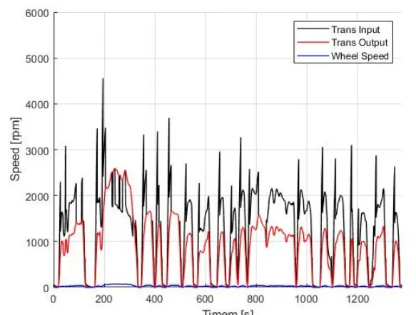
Plot the time trace for engine. transmission input, transmission output and wheel speed on one plot.
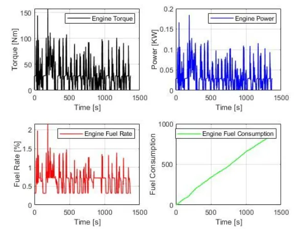
using subplots plot engine torque, engine power. fuel rate and fuel consumption.
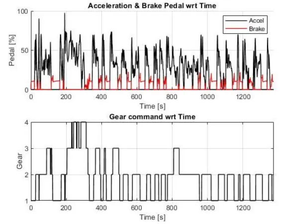
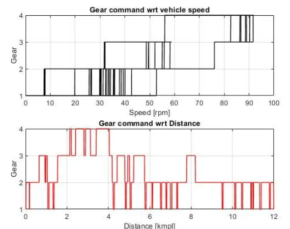
Again using subplots we have to plot accelerator and brake pedal, gear command, vehicle desired and actual speed, vehicle distance.
On the engine fuel map we have to plot engine operating points.
We have to generate plots for both dive cycles.
We have to do Study of Conventional vehicle simulink model and to create graphs.

CONVENTIONAL VEHICLE

It uses IC engine fueled by deisel to power the wheels.The principle of heat released is employed by heat engine for combustion.In the combustion chamber a gas is expanded which pushes against piston thereby creating force and torque.In the engine the chemical energy of fuel is getting converted into heat. It provides useful work.Mainly petroleum fuels are employed.

In our project a 4 stroke reciprocating engine.The engines are normally represented by thermodynamic cycles.The thermodynamic cycle consist of otto cycle and diesel cycle. otto cycle is employed for SI engines.THe diesel cycle is employed for CI engines.

ENERGY AND PERFORMANCE OF ENGINE.

In this system power demand have to be supplied by powertrain.The power demand on the wheels is also indicated by power on wheels.

CONVENTIONAL POWERTRAIN EFFICIENCY

The engine converts chemical energy to mechanical energy thereby power is getting generated.The process employed is combustion.The energy input is fuel consumption and it has a efficiency.

INSTANTANEOUS FUEL CONSUMPTION

It deals with the modeling of multi domain systems through the use of a unified approach based on a ordinary differential and algebraic equation describing the static and dynamic effects.

Each systems has are two generalised variables

1] Efforts:- It is generalised force variable, ex- torque, force, voltage, heating value.

2] Flow:- It is the generalised flow/velocity variable. ex:- velocity, current, mass flow rate.

MATLAB CODE

The code will load all aribles needed for running the SIMULINK model.The cycle selection is also done.The initializing script is run before vehicle dynamics model.

BLOCK DIAGRAMS

We will see block diagram of all subsystem one by one.In the question the engine used is of a a typical midsize car with a 1.9L engine and a 4-speed automatic transmission. Transmission shift map and controller is taken from Matlab/Simulink example database.

BLOCK DIAGRAM OF DRIVER CONTROLLER AND VEHICLE PLANT

VEHICLE PLANT SUBSYSTEM

SIMULINK MODEL FOR DRIVER UNIT

SIMULINK MODEL FOR CONTROLLER UNIT

It is the brain of the vehicle which represents control units. It is based on the inputs from the driver.It generates torque,desired transmission gear and brake torque.The powertrain block represents the drive train of the vehicle.

IDLE SPEED CONTROLLER SIMULINK MODEL

SIMULINK MODEL FOR ENGINE

SIMULINK FOR ENGINE CONTROL UNIT

SIMULINK MODEL FOR TRANSMISSION UNIT

To control the gears a steady flow variable is used.The order employed can be ascending or descending with respect to time,speed and distance. The lock diagram is depicted below.

SIMULINK MODEL FOR TORQUE CONVERTER

SIMULINK FOR POWER TRAIN

It will pass through all the components that converts power to movement.is includes the engine, transmission, driveshaft, differentials, axles; basically anything from the engine through to the rotating wheels.To model fuel consumption a map based model is employed.It depends on maximum and minimum torque.In these model we take engine torque, gear selector from controller for transmission of gear ratio. We will multiply the ratio with transmission torque, positive, negative torque that gives transmission input speed.The torque converter in the transmission system will connect engine with the transmission system.

SIMULINK MODEL FOR WHEELS

SIMULINK MODEL FOR DIFFERENTIAL

The output is taken from the transmission. This is then multiplied by differential ratio and to multiply the axle torque.The magnitude of axial torque is less than the transmission torque.In the model depicted below the transmission torque is taken from the differential and brake torque from the controller. The tractive force is obtainedfrom brake torque when it is subtracted and multiplied with rolling radius.The wheel speed is velocity.

SIMULINK MODEL FOR VEHICLE DYNAMICS

The Simulink model of vehicle is depicted below. The input is vehicle speed and the output obtained is vehicle velocity.We will also obtain the distance travelled by the vehicle.

UDDS CYCLE AND HWFET CYCLE

1) UDDS CYCLE

MATLAB CODE

POWER VS TIME FOR UDDS CYCLE

ENERGY VS TIME FOR UDDS CYCLE

2) HWFET CYCLE

MATLAB CODE

POWER VS TIME

ENERGY VS TIME

MATLAB CODE

%%Plotting vehicle characteristics time trace transmission IN/OUT and Wheel Speed

figure (1)

hold on

grid on

plot (Time, Trans_In_Spd, 'linewidth', 1, 'Color', 'black');

plot (Time, Trans_out_Spd, 'linewidth', 1, 'Color', 'red');

plot (Time, Wheel_Speed, 'linewidth',1, 'color', 'blue')

ylabel('Speed [rpm]')

xlabel('Timem [s]')

xlim([0, Time (end)]);

ylim([0,6000]);

legend('Trans Input', 'Trans Output', 'Wheel Speed');

%%Plotting vehicle characteristics time trace to Engine speed, Engine Torque, Engine Power,

% And Engine fuel rate, Engine fuel consumption

% Data conversion from Double Timeseries

Eng_spd=Eng_Spd.Data(:,1); % engine speed

Eng_trq= Eng_Trq.Data(:,1); % engine torque

Eng_pwr=Eng_Pwr.Data(:,1); % engine power

Eng_fuel_rate=Eng_Fuel_Rate.Data(:,1); % engine fuel rate

Eng_fuel_consumption = Eng_Fuel_Consump.Data(:,1); % engine fuel consumption

Veh_dist= Veh_Dist.Data(:,1); % vehicle distance.

veh_spd=Veh_Spd.Data(:,1); % vehicle speed

% Plotting Engine speed, Engine Torque, Engine Power, Engine fuel rate, Engine fuel consumption wrt

figure (2)

subplot (2,2,1)

plot(Time, Eng trq,'linewidth, 1,'color','black')

xlabel('Time [s]')

ylabel('Torque [Nm]')

legend('Engine Torque')

grid on

subplot (2,2,2)

plot(Time, Eng_pwr, 'linewidth',1, 'color', 'blue')

xlabel('Time [s]')

ylabel('Power [KW]')

legend('Engine Power')

grid on

subplot (2,2,3)

plot(Time, Eng_fuel_rate, 'linewidth',1, 'color', 'red')

xlabel( 'Time [s]')

ylabel('Fuel Rate [%]')

legend('Engine Fuel Rate')

grid on

subplot(2,2,4)

plot (Time,Eng_fuel consumption, 'linewidth',1, 'color', 'green')

xlabel('Time [s]')

ylabel('Fuel Consumption')

legend('Engine Fuel Consumption')

grid on

% Plotting fuel economy Vs Engine Fuel consumption

figure(3)

plot(Eng_fuel_consumption, Eng_fuel_rate, 'color', 'r')

xlabel('Fuel_consumption')

ylabel('Fuel_Rate [%]')

title('Fuel economy Vs Fuel consumption')

grid on

% Potting Accelerator pedal, Brake pedal and gear command with respect to time

figure(4)

subplot (2,1,1)

hold on

plot(Time, Acc_Pdl, 'linewidth', 1, 'Color', 'black');

plot (Time, Brk_Pdl, 'linewidth', 1, 'color', 'red');

xlabel('Time [s]');

ylabel('Pedal [%]');

xlim([0, Time(end)]);

grid on

legend( 'Accel', 'Brake');

title('Acceleration & Brake Pedal wrt Time')

subplot (2,1,2)

plot(Time, Gear_Cmd, 'linewidth', 1, 'Color', 'black');

xlim([0, Time(end)]);

xlabel('Time [s]');

ylabel('Gear');

grid on

title('Gear command wrt Time')

figure (5)

subplot (2,1,1)

plot (Veh_spd, Gear_Cmd, 'linewidth', 1, 'color', 'black');

xlabel('speed [rpm]');

ylabel('Gear');

title('Gear command wrt vehicle speed')

subplot (2,1,2)

plot (Veh_dist, Gear_Cmd, 'linewidth', 1, 'Color', 'red');

xlabel('Distance [kmpl]');

ylabel('Gear');

grid on

title('Gear command wrt Distance')

%% Plotting engine operating points on engine fuel map

figure('Name', 'Engine Operating Points');

hold on

grid on

title('Engine Operating Points', 'fontsize', 12);

pl=plot (Eng_map_spd*30/pi, Eng_max_trq, 'linewidth',2, 'color', 'r');

p2=line([Eng_map_spd (end)*30/pi Eng_map_spd (end) *30/pi], [0 Eng_max_trq(end)]);

set (p2, 'linewidth', 1, 'linestyle','--',' color', 'k');

p3=line([Eng_map_spd (1) 30/pi Eng_map_spd (1)*30/pi], [0 Eng_max_trq (1)]);

set(p3, 'linewidth', 1, 'linestyle', '--', 'color', 'k');

[c,h] = contour (Eng_map_spd '*30/pi, Eng_map_tra, Eng_fuel_map');

clabel (c,h);

xlabel('Engine Speed [rpm]');

ylabel('Engine Torque [Nm]');

title('Engine Fuel Consumption Map [g/s]');

legend ([p1 p3], ['Max Curve', 'Operating Points' });

axis ([Eng_map_spd (1) 30/pi Eng_map_spd (end) *30/pi e Eng_map_trq(end)]);

Plot of time trace for engine, transmission input, transmission output and wheel speed

Subplots of accelerator and brake pedal, gear command, vehicle desired and actual speed, vehicle distance .

PLOT OF ACCELERATOR,BRAKE PEDAL AND GEAR COMMAND

PLOT OF GEAR COMMAND DESIRED VS ACTUAL SPEED

Project 1

Ship work like this
in your own course.

Talk to a career counsellor

Ship work like thisin your own course.

Talk to a career counsellor

Ship work like this
in your own course.