Project 2

AIM :-Design and Develop a Simulink model to understand the Energy analysis of EVs on different driving cycles

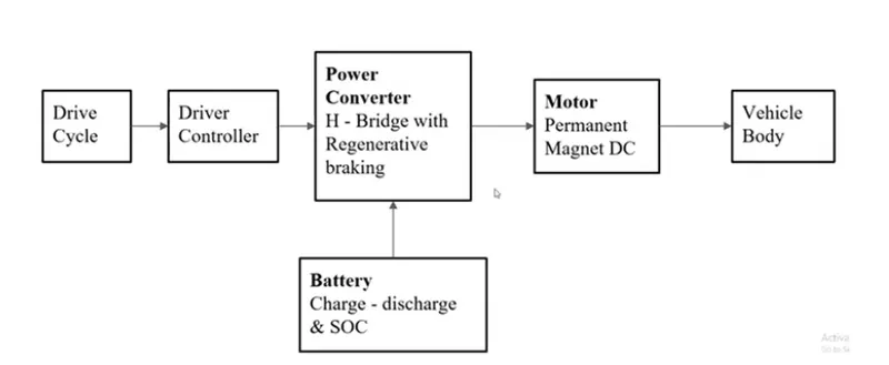
BLOCK DIAGRAM OF EV MODEL:

THEORY:-

Electric vechicles operates on electric motor instead of an IC engine that generates power by burning a mix of fuel and air. This is seen as a possible replacement of the existing traditional vehicle technology, in wake of the rising pollution, global warming, fossil depletion, etc. Amid the rising carbon footprint of fuel-based vehicles, a lot of vehicle manufacturers such as TATA Motors, Mahindra, Toyota Kirloskar, Ola Electric, etc, have made heavy advances towards the technology. Big players like Tesla, General Motors, Ford, Toyota, etc, have already worked on this technology since long in Europe and United States of America.

While some EVs used lead-acid or nickel-metal hydride batteries, the standard for modern battery electric vehicles is now considered to be lithium-ion batteries as they have greater longevity and are excellent at retaining energy, with a self-discharge rate of just 5% per month. Despite this improved efficiency, there are still challenges with these batteries as they can experience thermal runaway, which has, for example, caused fires or explosions in the Tesla Model S, although efforts have been made to improve the safety of these batteries.

• Drive cycle: This is the input given to the vehicle. There are different types of drive cycle based on the application we choose. In this vehicle is simulated for acceleration & deceleration for a particular type with the varying speed range.
• Driver controller: To drive the drive cycle as per the given condition, a driver controller is present to run the vehicle taking the input and feedback from to move from one place to another.
• Battery: This the powerhouse which supplies the energy required to drive the vehicle.
• Motor: It is the rotating device which converts the electrical energy in the form of current and voltage into the mechanical energy at the vehicle through a transmission system.
• Vehicle body: This is where the output is achieved via the motor power is transferred to the wheel considering the different forces and resistance and compare with the input drive cycle.

DESCRIPTION

VARIOUS BLOCKS USED IN EV DESIGN:

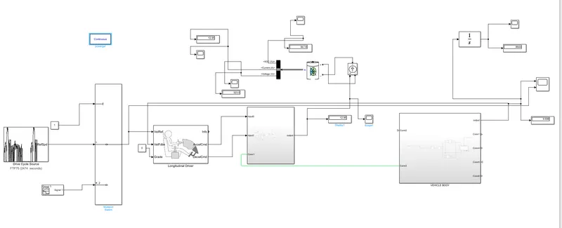
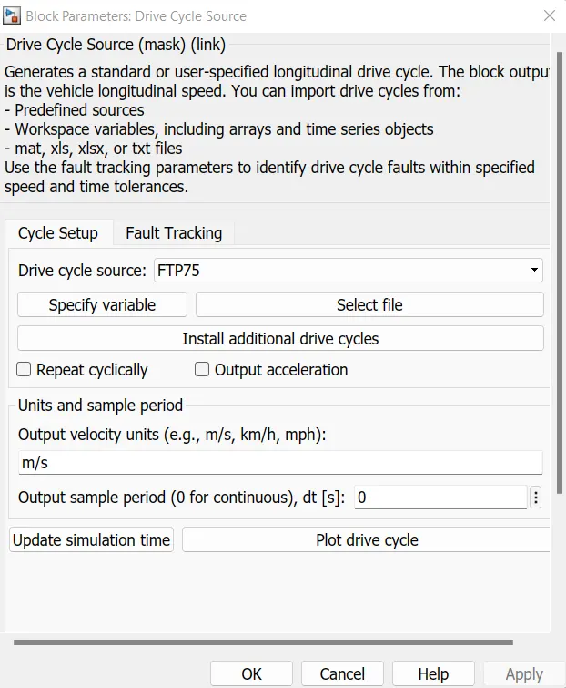
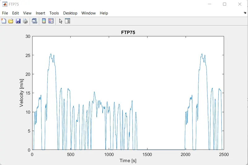
1. Drive Cycle Source:-The Drive Cycle Source block generates a standard or user-specified longitudinal drive cycle. The block output is the specified vehicle longitudinal speed, which you can use to:

• Predict the engine torque and fuel consumption that a vehicle requires to achieve desired speed and acceleration for a given gear shift reference.
• Produce realistic velocity and shift references for closed loop acceleration and braking commands for vehicle control and plant models
• Study, tune, and optimize vehicle control, system performance, and system robustness over multiple drive cycles.
• Identify the faults within tolerances specified by standardized tests.

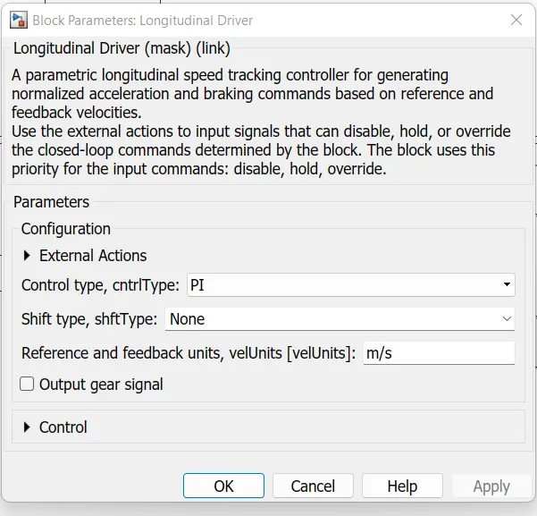
2. Longitudinal Drive:-The Longitudinal Driver block implements a longitudinal speed-tracking controller. Based on reference and feedback velocities, the block generates normalized acceleration and braking commands that can vary from 0 through 1. You can use the block to model the dynamic response of a driver or to generate the commands necessary to track a longitudinal drive cycle.

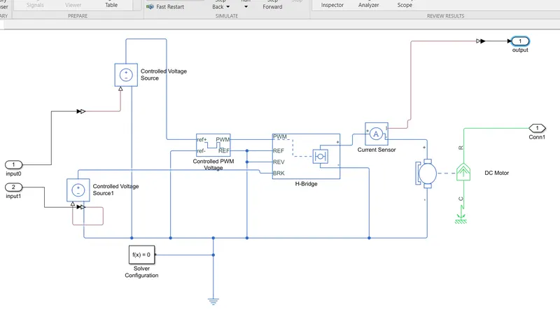
3. Controlled voltage source:-The Controlled Voltage Source block represents an ideal voltage source that is powerful enough to maintain the specified voltage at its output regardless of the current flowing through the source. The output voltage is V = Vs, where Vs is the numerical value presented at the physical signal port.

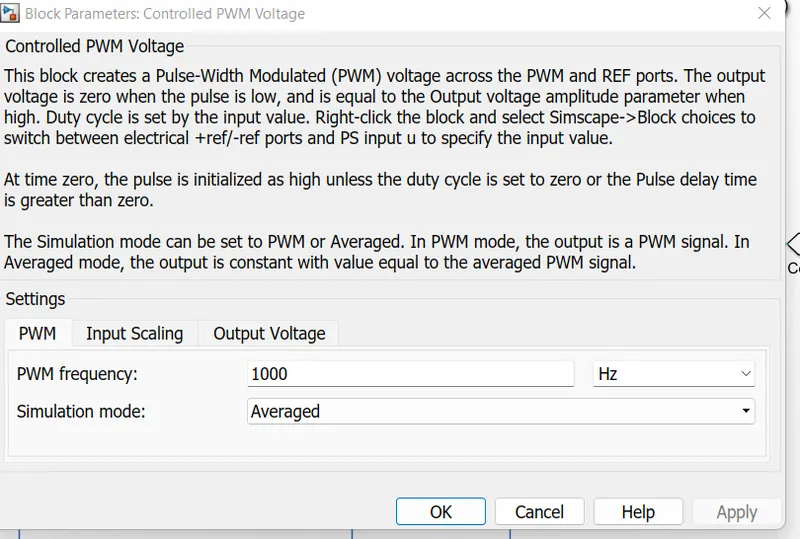
4. Controlled PWM voltage block:-The Controlled PWM Voltage block represents a pulse-width modulated (PWM) voltage source. The ports represented as

• Electrical input ports — The block calculates the duty cycle based on the reference voltage across its ref+ and ref- ports. This modelling variant is the default.
• PS input — Specify the duty cycle value directly by using an input physical signal port.

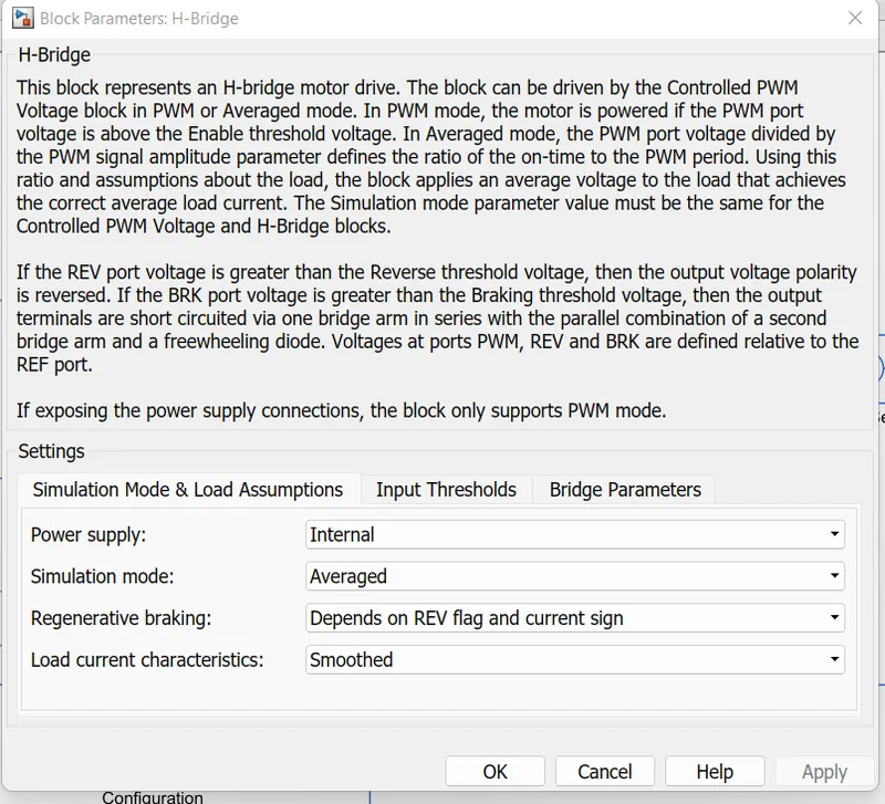
5. H–bridge:The block can be driven by the Controlled PWM Voltage block in PWM or Averaged mode. In PWM mode, the motor is powered if the PWM port voltage is above the Enable threshold voltage. In Averaged mode, the PWM port voltage divided by the PWM signal amplitude parameter defines the ratio of the on-time to the PWM period. Using this ratio and assumptions about the load, the block applies an average voltage to the load that achieves the correct average load current. The Simulation mode parameter value must be the same for the Controlled PWM Voltage and H-Bridge blocks

6. Current sensor:-The block represents an ideal current sensor, that is, a device that converts current measured in any electrical branch into a physical signal proportional to the current. Connections + and - are conserving electrical ports through which the sensor is inserted into the circuit. Connection I is a physical signal port that outputs current value.

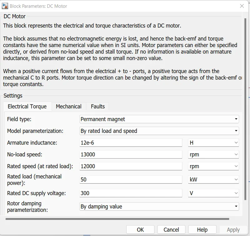
7. DC motor:-This block represents the electrical and torque characteristics of a DC motor. The block assumes that no electromagnetic energy is lost, and hence the back-emf and torque constants have the same numerical value when in SI units. Motor parameters can either be specified directly, or derived from no-load speed and stall torque. If no information is available on armature inductance, this parameter can be set to some small non-zero value. When a positive current flows from the electrical + to - ports, a positive torque acts from the mechanical C to R ports. Motor torque direction can be changed by altering the sign of the back-emf or torque constants.

8. Controlled Current Source:-The controlled current source block converts the Simulink input signal into an equivalent current source. The generated current is driven by the input signal of the block. The positive current direction is as shown by the arrow in the block icon. We can initialize the Controlled Current Source block with a specific AC or DC current. If we want to start the simulation in steady state, the block input must be connected to a signal starting as a sinusoidal or DC waveform corresponding to the initial values.

9. Battery:-The battery block represents a simple batery model. The block has four modeling variants, accessible by right-clicking the block in your block diagram and then selecting the appropriate option from the context menu, under Simscape > Block choices:

• Un-instrumented | No thermal port — Basic model that does not output battery charge level or simulate thermal effects. This modelling variant is the default.
• Un-instrumented | Show thermal port — Model with exposed thermal port. This model does not measure internal charge level of the battery.
• Instrumented | No thermal port — Model with exposed charge output port. This model does not simulate thermal effects.
• Instrumented | Show thermal port — Model that lets you measure internal charge level of the battery and simulate thermal effects. Both the thermal port and the charge output port are exposed.

10. Mechanical Rotational Reference:-The Mechanical Rotational Reference block represents a reference point, or frame, for all mechanical rotational ports. All rotational ports that are rigidly clamped to the frame (ground) must be connected to a Mechanical Rotational Reference block.

11. Electrical Reference:-The Electrical Reference block represents an electrical ground. Electrical conserving ports of all the blocks that are directly connected to ground must be connected to an Electrical Reference block. A model with electrical elements must contain at least one Electrical Reference block.

12. Solver Configuration:Each physical network represented by a connected Simscape block diagram requires solver settings information for simulation. The Solver Configuration block specifies the solver parameters that your model needs before you can begin simulation. Each topologically distinct Simscape block diagram requires exactly one Solver Configuration block to be connected to it.

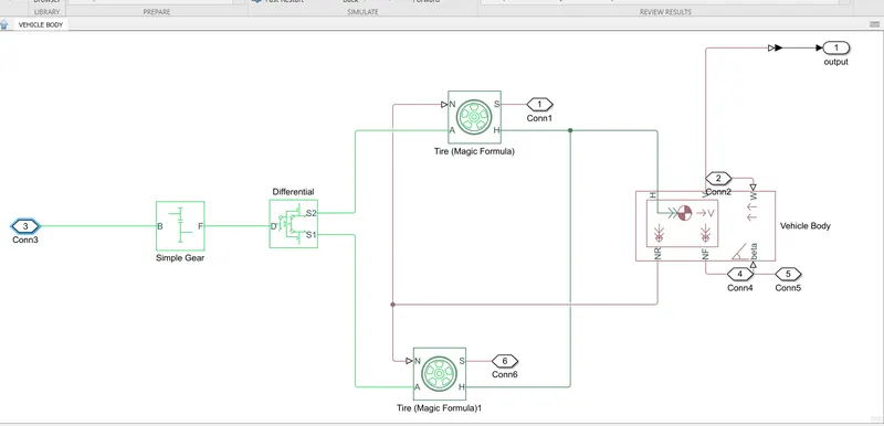
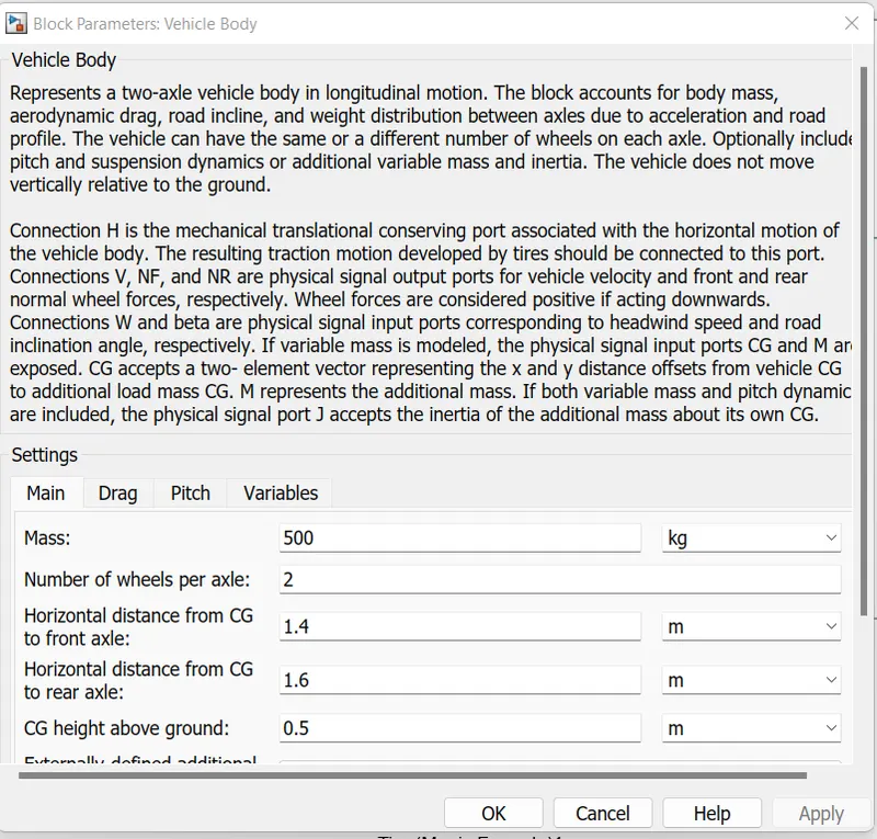
13. Vehicle Body:-The Vehicle Body block represents a two-axle vehicle body in longitudinal motion. The vehicle can have the same or a different number of wheels on each axle. For example, two wheels on the front axle and one wheel on the rear axle. The vehicle wheels are assumed identical in size. The vehicle can also have a centre of gravity (CG) that is at or below the plane of travel. The block accounts for body mass, aerodynamic drag, road incline, and weight distribution between axles due to acceleration and road profile. Optionally include pitch and suspension dynamics. The vehicle does not move vertically relative to the ground. The block has an option to include an externally-defined mass and an externally-defined inertia. The mass, inertia, and centre of gravity of the vehicle body can vary over the course of simulation in response to system changes.

14. Tire (Magic Formula):-The Tire (Magic Formula) block models a tire with longitudinal behaviour given by the Magic Formula, an empirical equation based on four fitting coefficients. The block can model tire dynamics under constant or variable pavement conditions.

15. Simple Gear:-The Simple Gear block represents a gearbox that constrains the connected driveline axes of the base gear, B, and the follower gear, F, to corotate with a fixed ratio that you specify. You choose whether the follower axis rotates in the same or opposite direction as the base axis. If they rotate in the same direction, the angular velocity of the follower, ωF, and the angular velocity of the base, ωB, have the same sign. If they rotate in opposite directions, ωF and ωB have opposite signs.
16. Discrete-Time Integrator:-Use the Discrete-Time Integrator block in place of the Integrator block to create a purely discrete model. With the Discrete-Time Integrator block, you can:

• Define initial conditions on the block dialog box or as input to the block
• Define an input gain (K) value
• Output the block state
• Define upper and lower limits on the integral
• Reset the state with an additional reset input

SIMULINK MODEL:-

SUBSYSTEM-

VEHICLE BODY:-

BLOCK PARAMETERS:-

OUTPUT:-

CONCLUSION:

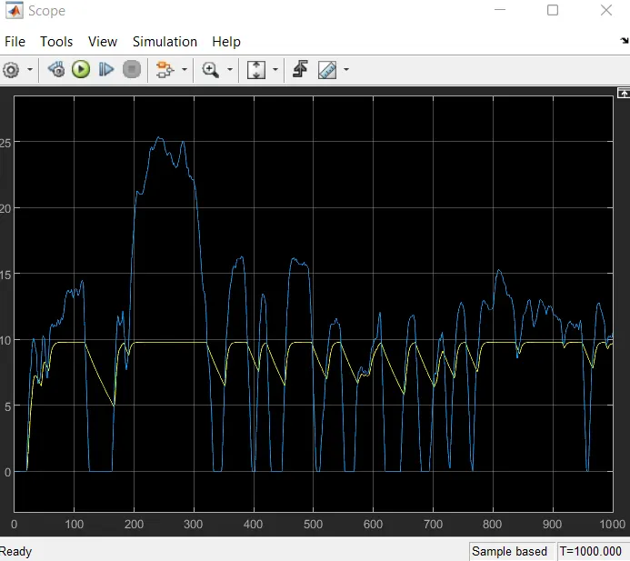
• In the speed comparison plots for all the drive cycles which are discussed in this study, the feedback/actual speed plot and the reference speed plot overlap each other almost completely but there are some regions where both speeds are different. It is when vehicle is decelerating. The reference speed graph falls sharply but actual/feedback speed doesn't. This is because of the inertia of the vehicle body. As the inertia of vehicle body is higher, it takes a longer duration for it to decelerate. That is why the overlapping is not 100%.
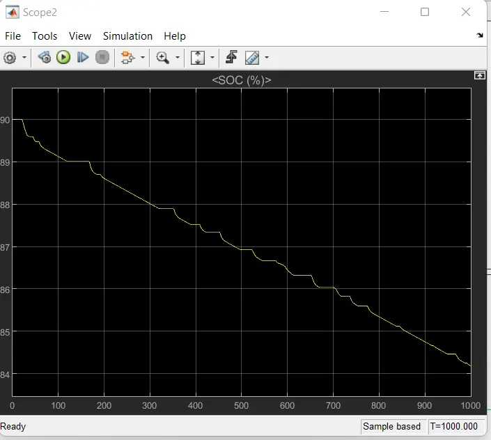
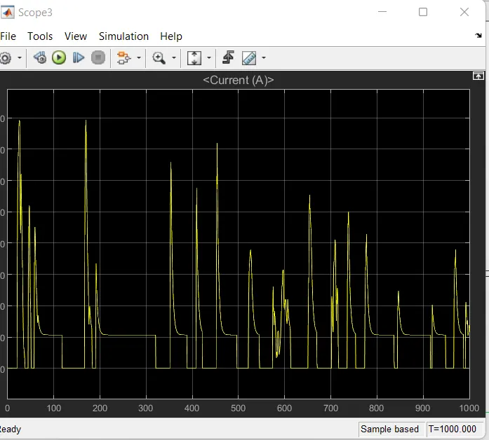
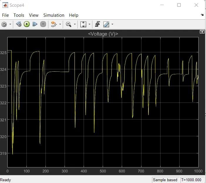
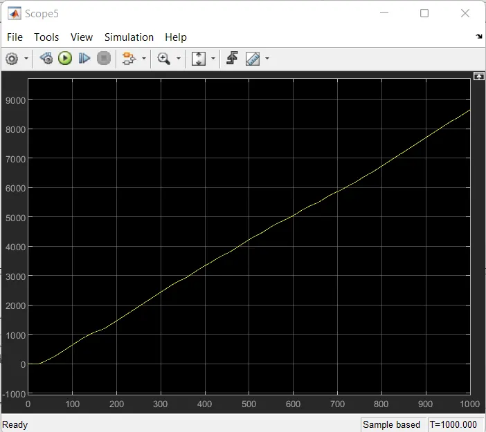
• In this study, BEV and its components have been simulated in order to investigate the energy flow, performance and efficiency. Good results for Battery Voltage, Current, and Power were shown by using MATLAB-Simulink.
• From the simulation we can say that the BEVs are much more efficient compared to thr traditional IC engine vehicles as they are non-polluting and the power loss is comparatively less.