Project 2
Development of a forward energy-based fuel consumption model of a P1 hybrid vehicle
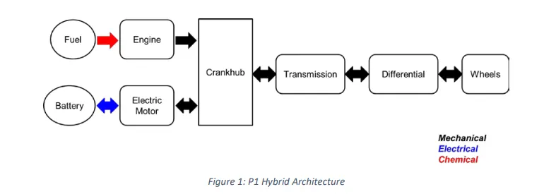
In the P1 hybrid vehicle model with the electric machine connected directly to the crankshaft, It is developed by Honda for their Integrated Motor Assist technology. The electric motor functions as a generator, during vehicle deceleration, as an engine starter, and as a motor during vehicle accelerations.
One of the biggest advantages of this technology is that the electric motor can provide higher torque since there is no slip. However, since there is no speed / torque ratio between the electric machine and crankshaft, the torque requirements on the electric motor is very demanding.
Initialization Code
This code is required to load all the required data to run the simulink model in the workspace.
%%%%%%%%%%%%%%%%%%%%%%%%%%%%%%%%%%%%%%%%%%%%%%%%%%%%%%%%%%%%%%%%%%%%%
%% Skill-Lync -> Hybrid Drives Development
% Project 2 - P1 Hybrid Vehicle Model
% By - Antarip Sinha

% Description:

%% Initialization File
% Initialization file for loading the variables for the P1 Hybrid Vehicle Model

%% Vehicle Parameters
M = 1500;       % Vehicle weight [kg]
Cr = 0.015;     % Rolling resistance coefficient
Rw = 0.35;      % Rolling radius [m]
Cd = 0.33;      % Drag coefficient
Af = 2;         % Frontal area [m2]
rhoa = 1.225;   % Air density [kg/m3]
Vwind = 0;      % Wind velocity [kmph]
g = 9.81;       % Gravitational acceleration [m/s2]
theta = 0;      % Slope [deg]
myu_road_tire = 1; % Coefficient of friction between tire - road interface

%% Powertrain Parameters
FDR = 3.73;                         % Final Drive Ratio / Diff Ratio
DiffEff = 0.99;                     % Differential efficiency (assumed independent of operating conditions)

NumGear = 4;                        % Number of gears in transmission
TransGear = [1:NumGear];            % Transmission Gears
TransRatio = [3.06, 1.62, 1, 0.7];  % Corresponding Transmission ratios
TransEff = 0.90;                    % Transmission efficiency (assumed independent of operating conditions)

TC_SR = [0, .5, .6, .7, .8, .87, .92, .94, .96, .97, 1];   % Torque Converter Speed Ratio (Matlab default) -> TurbSpd/PumpSpd
TC_TR = [2.232, 1.5462, 1.4058, 1.2746, 1.1528, 1.0732, 1.0192, 1, 1, 1, 1];   % Torque Converter Torque Ratio (Matlab default) -> TurbTrq/PumpTrq
TC_Cf = 1e-4 * [.72558, .66322, .63463, .59042, .51331, .4144, .29287, .22444, .12186, .04386, 0]; % Torque Converter Capacity Factor (Matlab default) -> PumpTrq/PumpSpd^2 [Nm/rpm^2]

load Vehicle_Data/Engine_data_1_9L_Saturn_95kW
load Vehicle_Data/Trans_Shift_map
load Vehicle_Data/EM_Honda_Insight_10kW
load Vehicle_Data/ESS_NiMH6


ESS_init_soc = 0.8;
ESS_soc_max = 0.9;
ESS_soc_min = 0.6;


%% Driver Parameters
Kp = 10;                    % P gain for driver PI model
Ki = 1;                     % I gain for driver PI model
Drive_Cycle_Select = 2;     % Drive cycle selection

% Drive cycle values in m/s

if Drive_Cycle_Select == 1
    load DriveCycles/UDDS;

elseif Drive_Cycle_Select == 2
    load DriveCycles/HWFET;

elseif Drive_Cycle_Select == 3
    load DriveCycles/FTP;

elseif Drive_Cycle_Select == 4
    load DriveCycles/US06;

elseif Drive_Cycle_Select == 5
    load DriveCycles/NEDC;

elseif Drive_Cycle_Select == 6
    load DriveCycles/WLTP;

end

time_end = cyc_time(end);
vel_end = cyc_vel(end);
Simulink Model
P1 hybrid vehicle model created in simulink
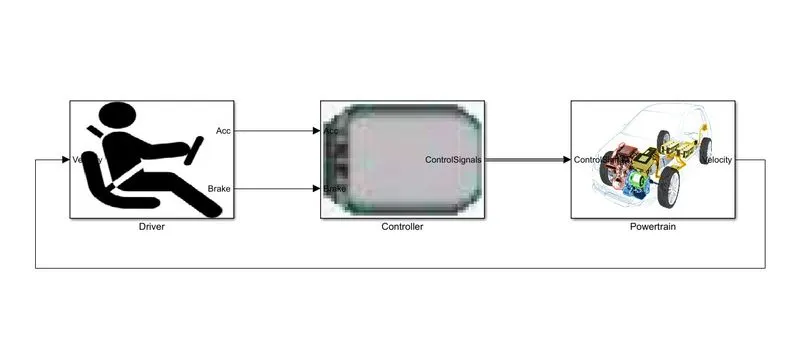
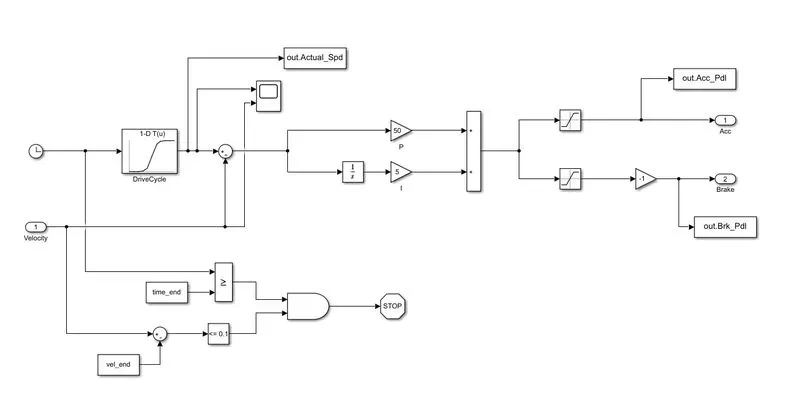
Driver
It contains a PI controller to get the accelerator and brake pedal signals depending upon the drive cycle requirements.
Controller
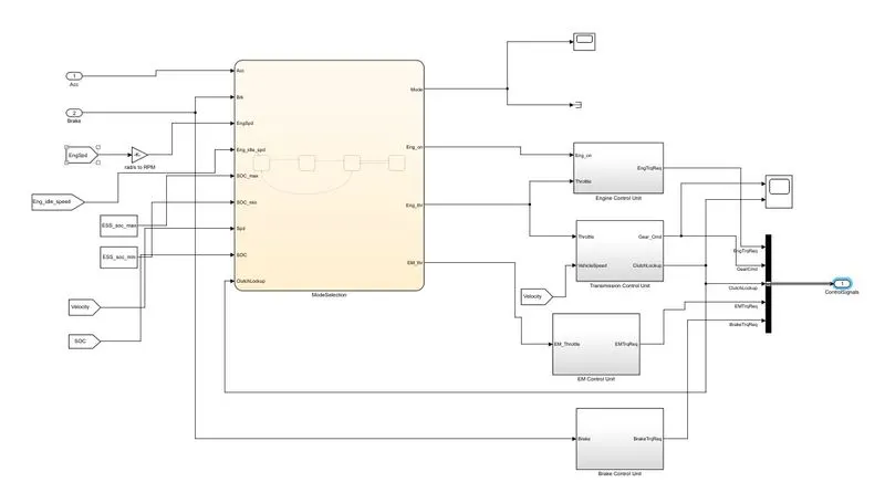
This works as the main computer of the vehicle. It generates desired engine and motor torque signals, gear signals, which goes to to the powertrain.
Mode Selection
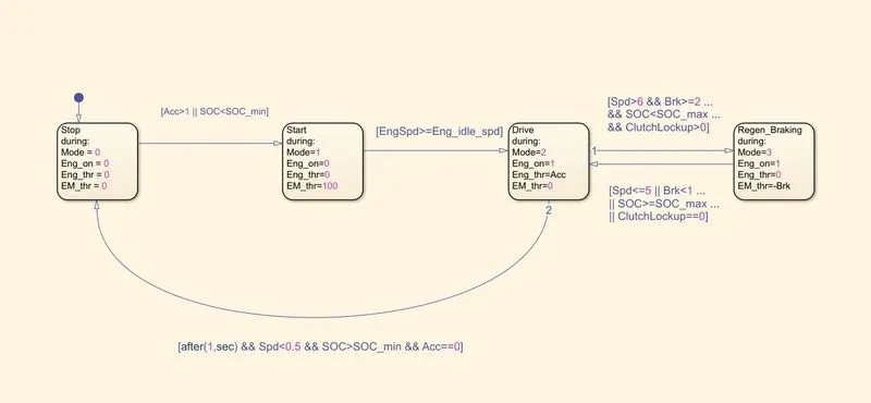
The chart has 4 states. those are Stop, Start, Drive and Regen Braking. Eng_on = 1 represents the engine is on, Eng_on = 0 represents the engine is off. Eng_thr and EM_thr are for the engine and EM throttle respectively
Engine Control Unit
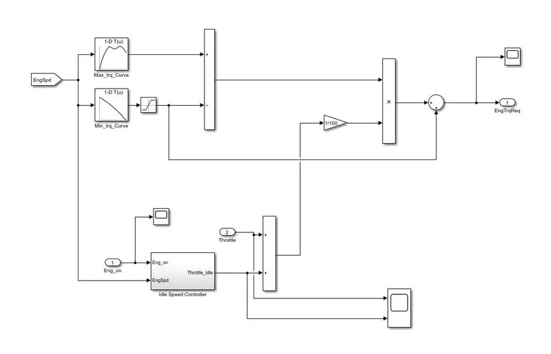
The idle speed controller keeps the speed above the idle speed and make sure that the engine is idling provided that the engine is on. The accelerator pedal from the driver unit provides the throttle signal as an input. It has two look up tables for maximum and minimum torque curves for various speed values. The input to the tables is the engine speed. This input along with the throttle and idle speed controller signals are multiplied together to get the required engine torque.
Transmission Control Unit
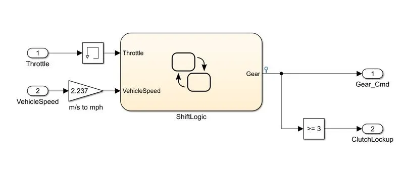
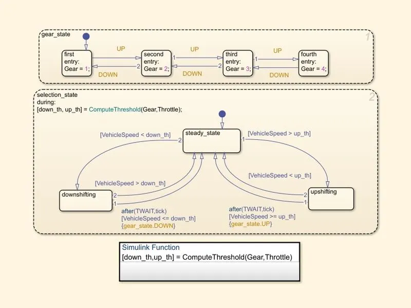
This state represents gear shifting by judging the throttle and vehicle speed.
Shift Logic
EM Control Unit
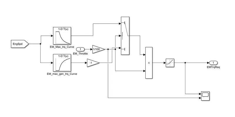
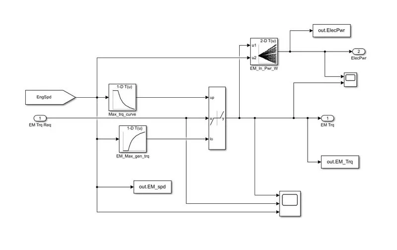
This control unit feeds the required Electric motor torque to the Power Train. Engine speed is the input in this control unit.
Brake Control Unit
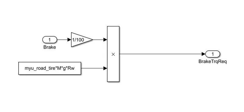
The brake torque is calculated analytically and multiplying it with the brake signal, the magnitude of the brake torque which is required is generated.
Power Train
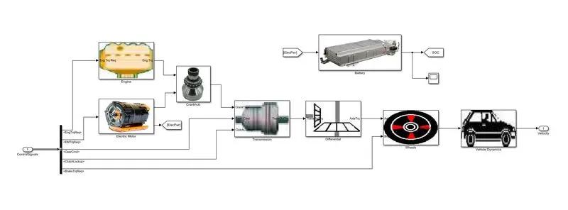
The Power Train block has model of all the mechanical components. Control signals from the controller block are fed into the respective models by a signal bus.
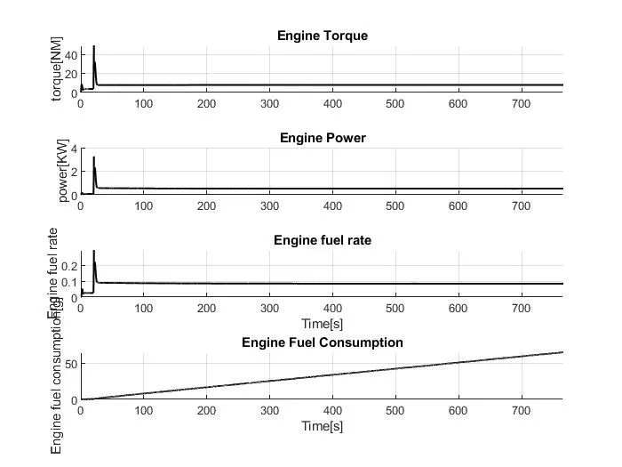
Engine
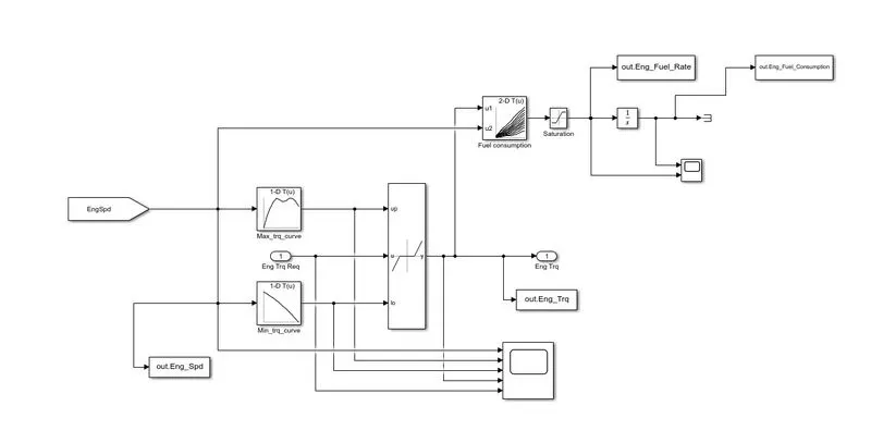
The look up table gives the Engine fuel rate and the integrator gives the Engine fuel consumption.
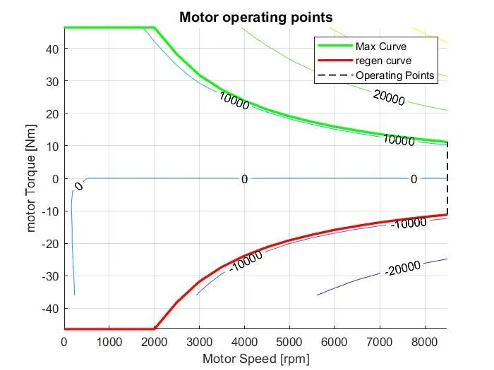
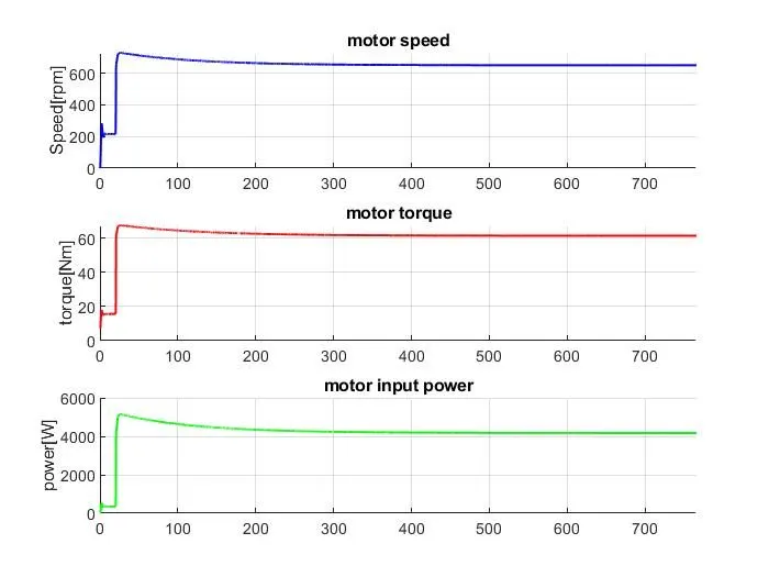
Electric Motor
Crank hub
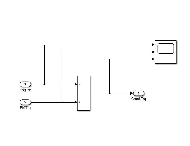
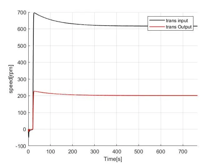
Transmission
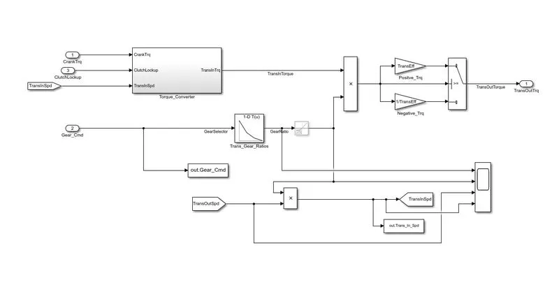
The Crank torque, Transmission speed and the clutch lock up signal go into the torque converter. The gear output signals are sent to the transmission gear ratio look up table. The gear ratio is then multiplied with the transmission torque and transmission efficiency to get the transmission output torque. The gear ratio is also multiplied with the transmission speed to get the transmission output speed.
Torque Converter
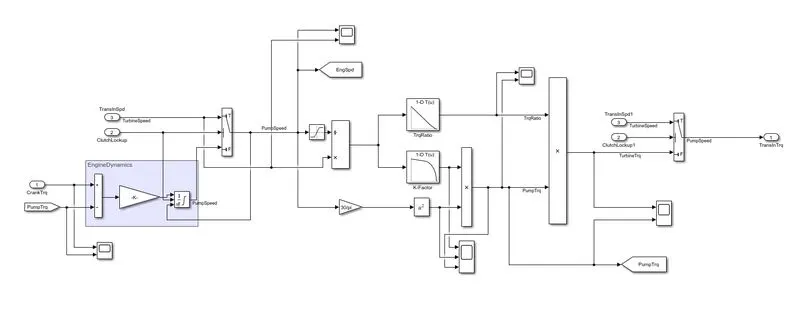
Differential
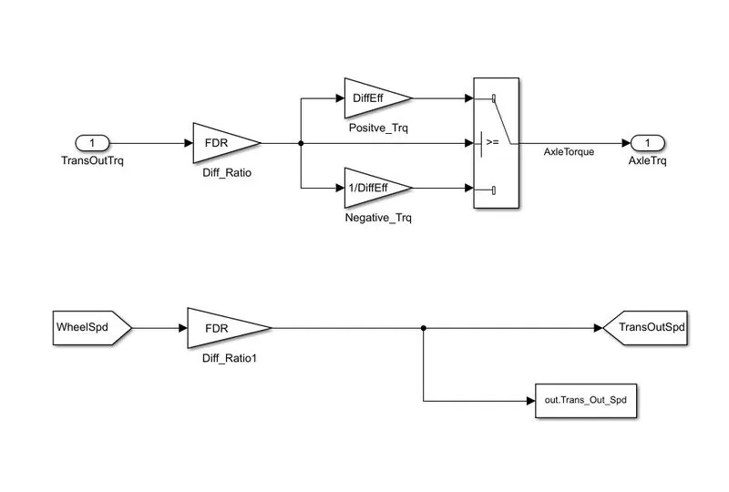
Wheels
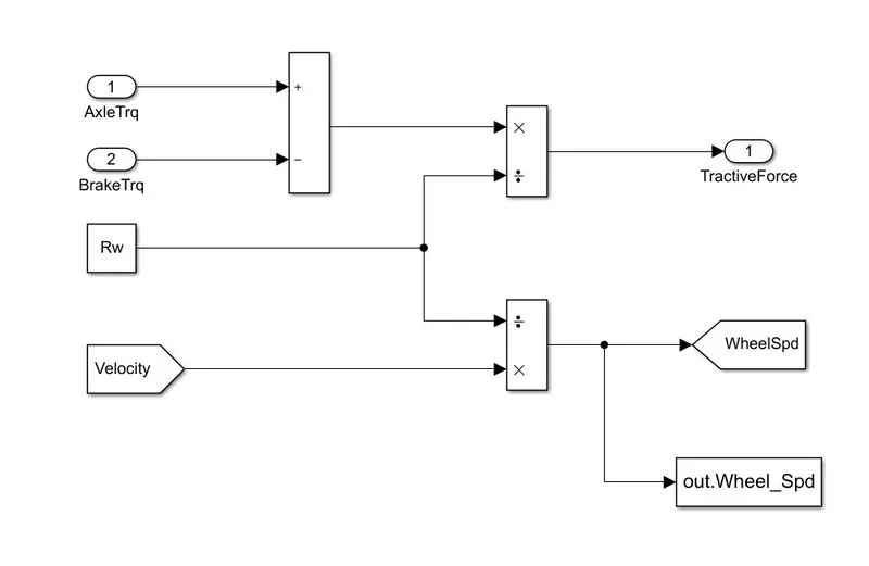
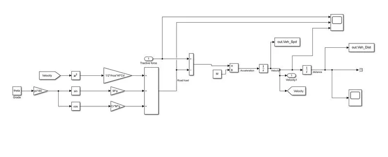
Vehicle Dynamics
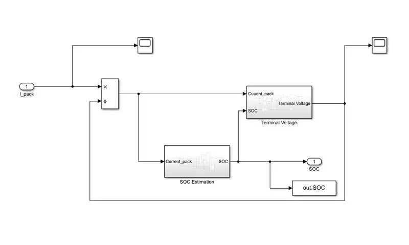
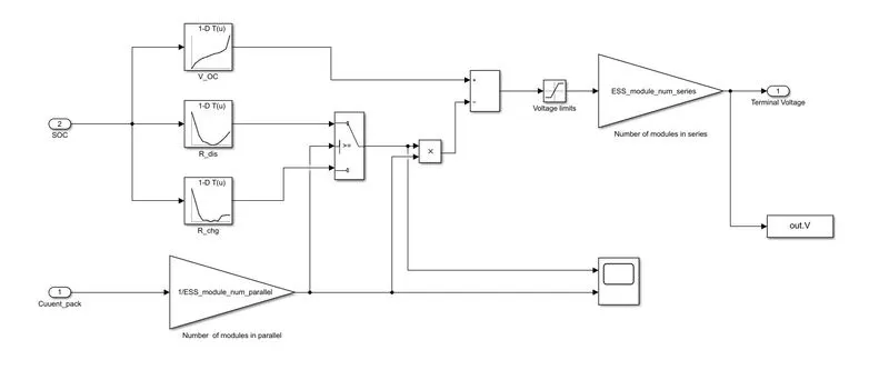
Battery Model
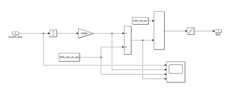
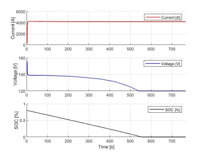
SOC Estimation
Terminal Voltage
Result
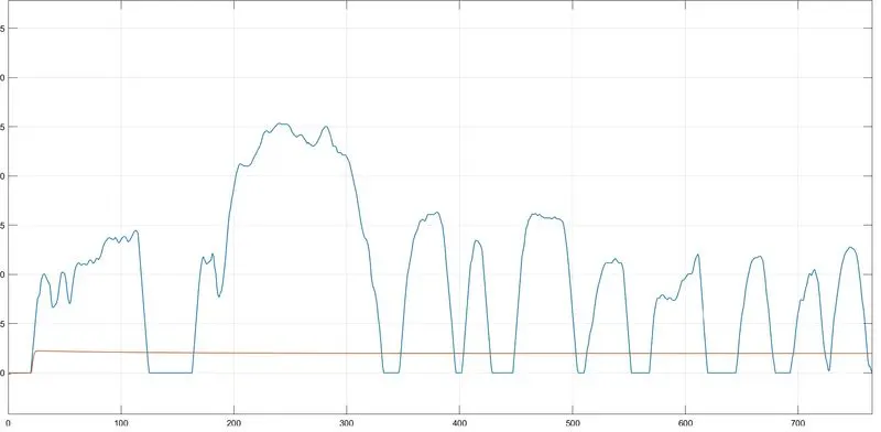
UDDS
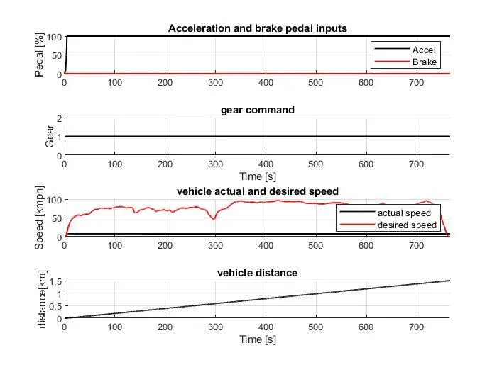
Actual speed vs Velocity
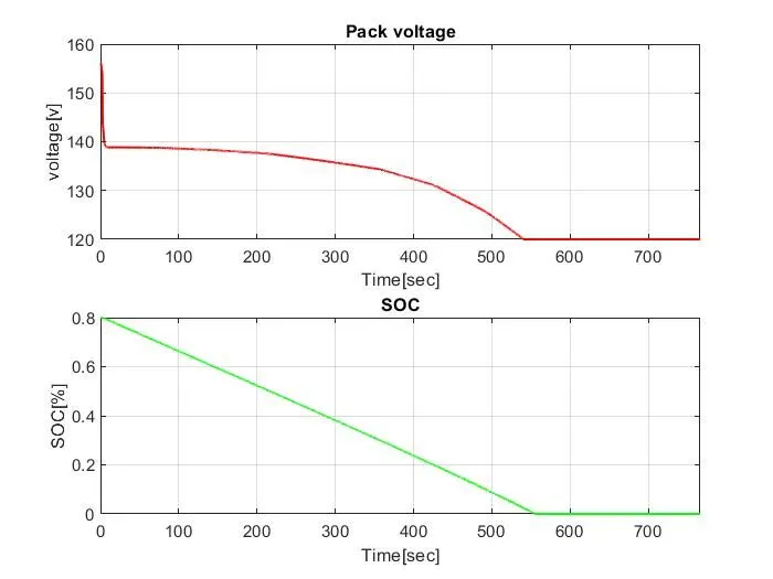
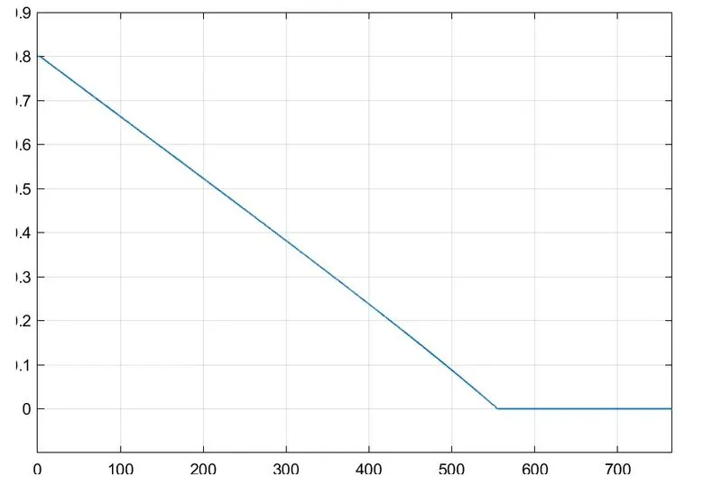
SOC
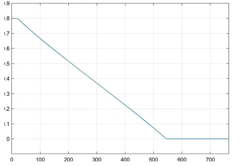
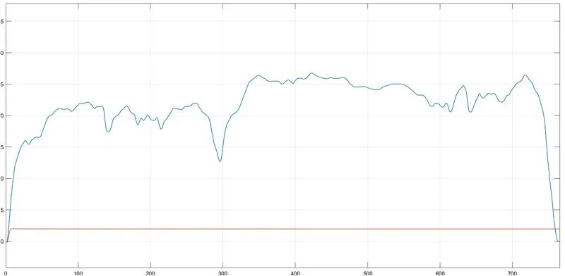
HWFET
Actual speed vs Velocity
SOC
Post Processing Code
%% Skill-Lync -> Hybrid Drives Development
% Project 2 - P1 Hybrid Vehicle Model
% By - Antarip Sinha

% Description:

%% Initialization File
% Initialization file for loading the variables for the P1 Hybrid Vehicle Model

%% Renaming variables
Time = out.tout;
Acc_Pdl = out.Acc_Pdl;          % Accelerator pedal [%]
Brk_Pdl = out.Brk_Pdl;          % Brake pedal [%]
Gear_Cmd = out.Gear_Cmd;        % Transmission gear
Trans_In_Spd = out.Trans_In_Spd*30/pi;  % Transmission input speed [rpm]
Trans_Out_Spd = out.Trans_Out_Spd*30/pi;% Transmission output speed [rpm]
Eng_Trq = out.Eng_Trq;          % Engine brake torque [Nm]
Eng_Spd = out.Eng_Spd*30/pi;    % Engine speed [rpm]
Eng_Fuel_Consump = out.Eng_Fuel_Consumption;    % Engine fuel consumption [g]
Eng_Fuel_Rate= out.Eng_Fuel_Rate;
Veh_Dist = out.Veh_Dist/1000;   % Distance traveled by vehicle [km]
Veh_Spd = out.Veh_Spd*18/5;     % Vehicle speed [kmph]
Actual_Spd=out.Actual_Spd*18/5;      % Actual speed in [kmph]
EMS=out.EM_spd./0.10472;
EM_Pwr= out.ElecPwr;
Wheel_Spd =out.Wheel_Spd*30/pi;  %Wheel Speed in [RPM]
Current_pack=out.Current_pack;  %Battery pack current in ampears
P=out.ElecPwr;
SOC=out.SOC;
V=out.V;
RS = out.RS;          % internal resistance
VOC = out.VOC;        % open circuit voltage


%% Data Analysis
Eng_Pwr = Eng_Spd.*pi./30.*Eng_Trq./1000;   % Engine brake power [kW]
rho_petrol = 0.7197;                    % Density of petrol [kg/L]
Eff=Eng_eff_map.*100;
Pwr=EM_inpwr_map./1000;
EMT=9.5488.*P./EMS;
kmpl = Veh_Dist(end)/(Eng_Fuel_Consump(end)/1000/rho_petrol);    % Fuel economy [kmpl]
Range=P(end)./(Eng_Fuel_Consump(end)*100/1000/rho_petrol);

%% Plotting vehicle characteristics time trace
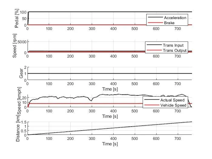
figure(1)
subplot(5,1,1)
hold on
grid on
plot(Time, Acc_Pdl, 'linewidth', 1, 'Color', 'black');
plot(Time, Brk_Pdl, 'linewidth', 1, 'Color', 'red');
ylabel('Pedal [%]')
xlim([0, Time(end)]);
legend('Acceleration','Brake');
subplot(5,1,2)
hold on
grid on
plot(Time, Trans_In_Spd, 'linewidth', 1, 'Color', 'black');
plot(Time, Trans_Out_Spd, 'linewidth', 1, 'Color', 'red');
ylabel('Speed [rpm]')
xlim([0, Time(end)]);
ylim([0, 6000]);
legend('Trans Input','Trans Output');
subplot(5,1,3)
hold on
grid on
plot(Time, Gear_Cmd, 'linewidth', 1, 'Color', 'black');
xlim([0, Time(end)]);
xlabel('Time [s]');
ylabel('Gear');
subplot(5,1,4)
hold on
grid on
plot(Time, Actual_Spd, 'linewidth', 1, 'Color', 'black');
plot(Time, Veh_Spd, 'linewidth', 1, 'Color', 'red');
xlim([0, Time(end)]);
xlabel('Time [s]');
ylabel('Speed [kmph]');
legend('Actual Speed','Vehicle Speed');
subplot(5,1,5)
hold on
grid on
plot(Time,Veh_Dist, 'linewidth', 1, 'Color', 'black');
xlim([0, Time(end)]);
xlabel('Time [s]');
ylabel('Distance [km]');

%% Plotting engine operating points on engine fuel map
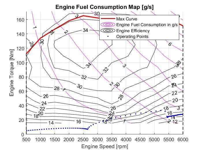
figure(2);
hold on
grid on
title('Engine Operating Points','fontsize',12);
p1=plot(Eng_map_spd*30/pi,Eng_max_trq,'linewidth',2,'color','r');
[c,h] = contour(Eng_map_spd'*30/pi,Eng_map_trq,Eng_fuel_map','m');
clabel(c,h);
[c1,h1] = contour(Eng_map_spd'*30/pi,Eng_map_trq,Eff','k');
clabel(c1,h1);
p2=plot(Eng_Spd*30/pi,Eng_Trq,'.','color','b');
p3=line([Eng_map_spd(end)*30/pi Eng_map_spd(end)*30/pi],[0 Eng_max_trq(end)]);
set(p3,'linewidth',1,'linestyle','--','color','k');
xlabel('Engine Speed [rpm]');
ylabel('Engine Torque [Nm]');
title('Engine Fuel Consumption Map [g/s]');
p4 = line([Eng_map_spd(1)*30/pi Eng_map_spd(1)*30/pi],[0 Eng_max_trq(1)]);
set(p4,'linewidth',1,'linestyle','--','color','k');
legend('Max Curve','Engine Fuel Consumption in g/s','Engine Efficiency','Operating Points');
axis([Eng_map_spd(1)*30/pi Eng_map_spd(end)*30/pi 0 Eng_map_trq(end)]);

%% Plotting Motor operating points
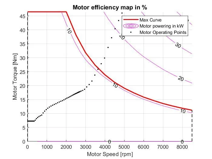
figure(3);
hold on
grid on
title('Motor Operating Points','fontsize',12);
p1=plot(EM_map_spd*30/pi,EM_max_trq,'linewidth',2,'color','r');
[c,h] = contour(EM_map_spd'*30/pi,EM_map_trq,Pwr','m');
clabel(c,h);
p2 = plot(EMS*30/pi,EMT,'.','color','b');
set(p2,'linewidth',1,'marker','.','color','k');
p3=line([EM_map_spd(end)*30/pi EM_map_spd(end)*30/pi],[0 EM_max_trq(end)]);
set(p3,'linewidth',1,'linestyle','--','color','k');
p4=line([EM_map_spd(1)*30/pi EM_map_spd(1)*30/pi],[0 EM_max_trq(1)]);
set(p4,'linewidth',1,'linestyle','--','color','k');
xlabel('Motor Speed [rpm]');
ylabel('Motor Torque [Nm]');
title('Motor efficiency map in %');
legend('Max Curve','Motor powering in kW','Motor Operating Points');
axis([EM_map_spd(1)*30/pi EM_map_spd(end)*30/pi 0 EM_map_trq(end)]);

%% Plotting power,voltage,SOC

figure(4);
subplot(3,1,1)
hold on
grid on
plot(Time, P, 'linewidth', 1, 'Color', 'r');
xlim([0, Time(end)]);
ylim([0, 6000]);
ylabel('Current [A]')
legend('Current [A]');
subplot(3,1,2)
hold on
grid on
plot(Time, V, 'linewidth', 1, 'Color', 'b');
xlim([0, Time(end)]);
ylabel('Voltage [V]')
legend('Voltage [V]');
subplot(3,1,3)
hold on
grid on
plot(Time, SOC, 'linewidth', 1, 'Color', 'k');
legend('SOC [%]');
xlim([0, Time(end)]);
xlabel('Time [s]');
ylabel('SOC [%]');


%% Plotting motor speed ,motor torque,motor input power

figure(5)
subplot(3,1,1)
hold on
grid on
plot(Time,EMS,'LineWidth',1,'Color','b');
ylabel('Speed[rpm]')
xlim([0,Time(end)]);
title('motor speed')

subplot(3,1,2)
hold on
grid on
plot(Time,EMT,'LineWidth',1,'Color','r');
ylabel('torque[Nm]')
xlim([0,Time(end)]);
title('motor torque')

subplot(3,1,3)
hold on
grid on
plot(Time,EM_Pwr,'LineWidth',1,'Color','g');
ylabel('power[W]')
xlim([0,Time(end)]);
title('motor input power')

%% Plotting Transmission input,Transmission output
figure(6)
hold on
grid on
plot(Time,Trans_In_Spd,'LineWidth',1,'Color','black');
plot(Time,Trans_Out_Spd,'LineWidth',1,'Color','red');
xlabel('Time[s]')
ylabel('speed[rpm]')
xlim([0,Time(end)]);
legend('trans input','trans Output');

%% Plotting Engine Torque,Engine Power,Engine fuel rate,Engine fuel consumption

figure(7)
subplot(4,1,1)
hold on
grid on
plot(Time,Eng_Trq,'LineWidth',1,'Color','black');
ylabel('torque[NM]')
xlim([0,Time(end)]);
title('Engine Torque')

subplot(4,1,2)
hold on
grid on
plot(Time,Eng_Pwr,'LineWidth',1,'Color','black');
ylabel('power[KW]')
xlim([0,Time(end)]);
title('Engine Power')

subplot(4,1,3)
hold on
grid on
plot(Time,Eng_Fuel_Rate,'LineWidth',1,'Color','black');
xlim([0,Time(end)]);
xlabel('Time[s]');
ylabel('Engine fuel rate');
title('Engine fuel rate')

subplot(4,1,4)
hold on
grid on
plot(Time,Eng_Fuel_Consump,'LineWidth',1,'Color','black');
xlim([0,Time(end)]);
xlabel('Time[s]');
ylabel('Engine fuel consumption[g]');
title('Engine Fuel Consumption')

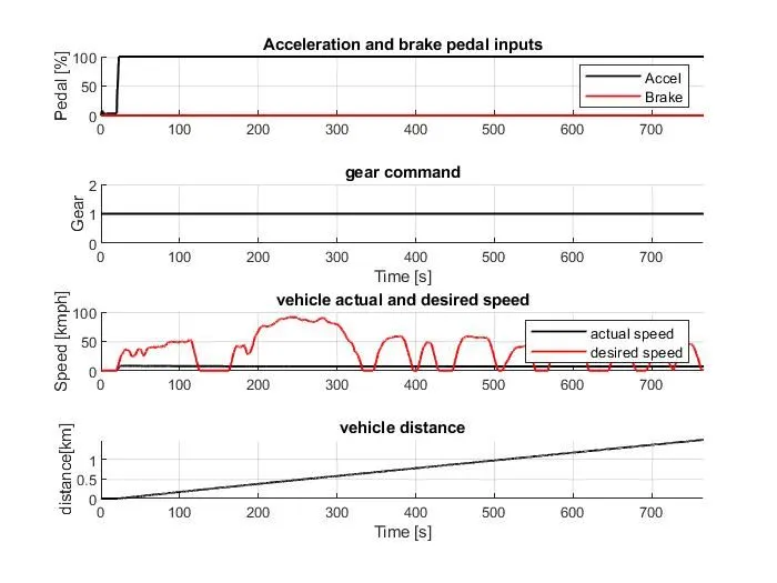
%% Plotting Acceleration, Brake inputs
figure(8)
subplot(4,1,1)
hold on
grid on
plot(Time, Acc_Pdl, 'linewidth', 1, 'Color', 'black');
plot(Time, Brk_Pdl, 'linewidth', 1, 'Color', 'red');
ylabel('Pedal [%]')
xlim([0, Time(end)]);
legend('Accel','Brake');
title('Acceleration and brake pedal inputs')

subplot(4,1,2)
hold on
grid on
plot(Time, Gear_Cmd, 'linewidth', 1, 'Color', 'black');
xlim([0, Time(end)]);
xlabel('Time [s]');
ylabel('Gear');
title('gear command')

subplot(4,1,3)
hold on
grid on
plot(Time, Veh_Spd, 'linewidth', 1, 'Color', 'black');
plot(Time, Actual_Spd, 'linewidth', 1, 'Color', 'red');
ylabel('Speed [kmph]')
xlim([0, Time(end)]);
legend('actual speed','desired speed');
title('vehicle actual and desired speed')

subplot(4,1,4)
hold on
grid on
plot(Time, Veh_Dist, 'linewidth', 1, 'Color', 'black');
xlim([0, Time(end)]);
xlabel('Time [s]');
ylabel('distance[km]');
title('vehicle distance')

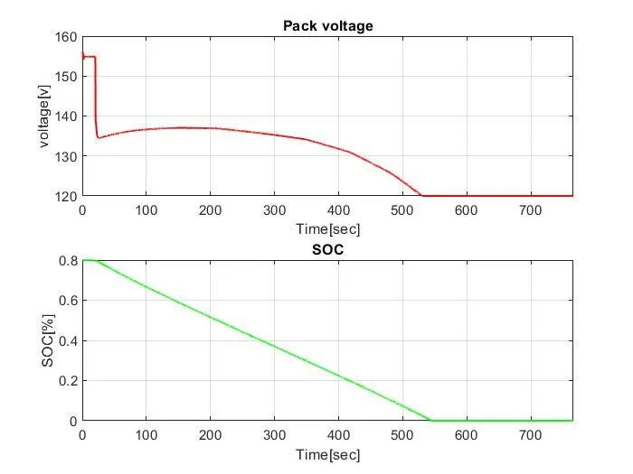
%% Plotting pack voltage, SOC

figure(9)
subplot(2,1,1)
plot(Time,V,'LineWidth',1,'Color','r');
xlabel('Time[sec]');
ylabel('voltage[v]');
title('Pack voltage')
xlim([0,Time(end)]);
grid on

subplot(2,1,2)
plot(Time,SOC,'LineWidth',1,'Color','g');
xlabel('Time[sec]');
ylabel('SOC[%]');
title('SOC')
xlim([0,Time(end)]);
grid on

%%Plotting Electric motor operating points

figure(10);
hold on
grid on
title('Electric motor Operating Points','fontsize',12);
p1=plot(EM_map_spd*30/pi,EM_max_trq,'linewidth',2,'color','g');
p4=plot(EM_map_spd*30/pi,EM_max_gen_trq,'LineWidth',2,'Color','r');
p2=line([EM_map_spd(end)*30/pi EM_map_spd(end)*30/pi],[EM_max_gen_trq(end) EM_max_trq(end)]);
set(p2,'linewidth',1,'linestyle','--','color','black');
p3=line([EM_map_spd(1)*30/pi EM_map_spd(1)*30/pi],[EM_max_gen_trq(1) EM_max_gen_trq(1)]);
set(p3,'linewidth',1,'linestyle','--','color','black');
[c,h] = contour(EM_map_spd'*30/pi,EM_map_trq,EM_inpwr_map');
clabel(c,h);
xlabel('Motor Speed [rpm]');
ylabel('motor Torque [Nm]');
title('Motor operating points');
legend([p1 p4 p3],{'Max Curve','regen curve','Operating Points'});
xlim([EM_map_spd(1)*30/pi EM_map_spd(end)*30/pi]);
ylim([EM_max_gen_trq(1) EM_max_trq(1)]);


%Display calculated fuel economy of vehicle
fprintf('\nFuel economy [km/L] : %f kmpl',kmpl);
fprintf('\nElectrical drive Range [km] : %f km',Range);
Plots
UDDS
Fuel economy numbers

HWFET
Fuel economy numbers