Project 2

Aim:tTo understand the functionality of a P1 hybrid and be able to model it.Honda Insight motor and battery are considered for this project.

Task:

The task of this project is to quantify the improvement in fuel economy numbers for the hybrid vehicle (kmpl), compared to the conventional vehicle, on the urban cycle (UDDS) and highway cycle (HWFET). Also, to analyze and understand the vehicle operating points in terms of engine and motor speed, torque, transmission speeds, pedal positions, gear, distance traveled, battery voltage, current, SoC etc.

a. Tabulate the fuel economy numbers (kmpl) for UDDS and HWFET cycle. Compare these numbers with the baseline numbers for conventional vehicle model from Project 1.
b. Plot the time trace for engine, transmission input, transmission output and wheel speed on one plot.
c. Plot engine torque, engine power, fuel rate and fuel consumption using subplots.
d. Plot accelerator and brake pedal, gear command, vehicle desired and actual speed, vehicle distance using subplots.
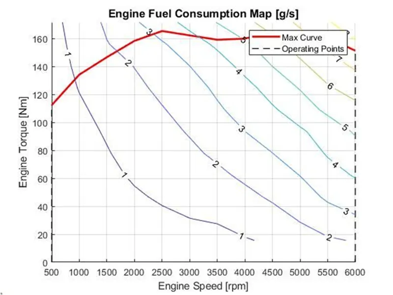
e. Plot the engine operating points on the engine fuel map.
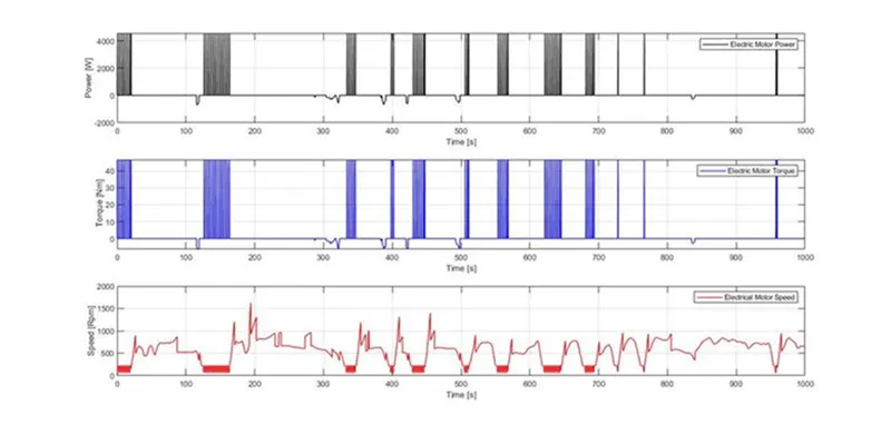
f. Plot motor speed, torque, motor input power using subplots.
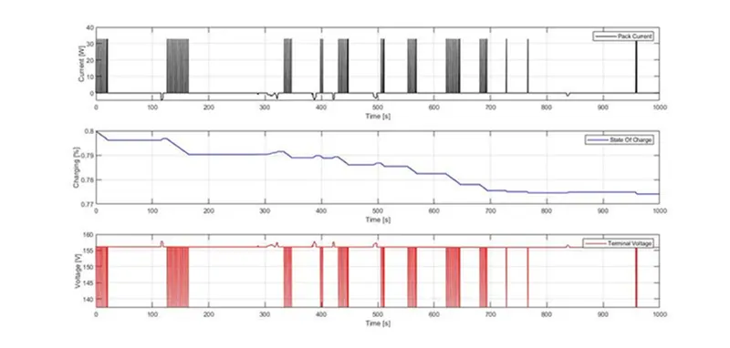
g. Plot pack voltage, current and SoC using subplots.
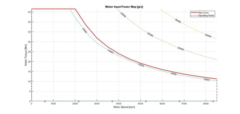
h. Plot the motor operating points on the motor input power map, with the motor max motoring and generating torque curves.
i. Write down appropriate brief comments on each of these plots, describing the vehicle behavior throughout the drive cycle.
j. Generate the plots for both drive cycles

Introduction of P1 architecture:

P1 Mild Hybrid Electric Vehicle:-

The P1 architecture its one of the type of architecutre with the electric machine connected directly to the crankshaft, is the solution adopted by Honda on their first generation Integrated Motor Assist (IMA) technology. In this electric motor functions as a generator, during vehicle deceleration, as an engine starter, and as a motor (to assist the engine) during vehicle accelerations. It has one of the biggest advantage of this solution is that the electric motor can provide higher torque than the BiSG, since there is no belt limitation (due to slip). However, since there is no speed / torque ratio between the electric machine and crankshaft, the torque requirements on the electric motor can be quite demanding.

There are two examples of P1 MHEV architectures are:

• Honda Insight Hybrid 2009 (with Integrated Motor Assist technology)
• Mercedes Benz S400 Bluehybrid 2010

For example, the main characteristics of the P1 MHEV.

1] ELectric Machine Performance:-

• Maximum torque up to 34 Nm.
• Maximum power: 10KW
• Efficiency: Up to 94 Percent

2] Hybrid Modes:-

• Idle stop and stop
• Moving stop and start
• Engine load shift
• Torque assist
• Torque boost
• Energy recuperation
• Brake generation

3] Advantages:-

• Higher efficiency
• The 12V starter can be removed

4] Disadvantages:-

• Output torque limited by thje size of the elctric machine
• Energy recuperation affected by engine friction losses
• High impact on existing vehicle architecture
• Higher overall cost of the electrical components
• Air cooling not possible for electric machine

5] Overall charcteristics:-

• Toruqe Boosting capacity is High
• Electrical energy recuperation is Medium
• Driveability improvements is Medium
• Electrical Creep/drive is Possible

In this model We use Forward Model:-It also known as dynamic simulation. its used for detailed simulations. In this model force/torque/power is the input and the vehicle state variable velocity and acceleration are outputs. The models and simulatios are more realistic due to phhysical casualty hence appropriate for control development. There is feedback loop to meet the desired vehicle state. It is mainly useful for simulate a vehicle on a driving cycle to analyse the dynamic behaviour of the system helps significantly in control development.

• Matlab Code:

%%%%%%%%%%%%%%%%%%%%%%%%%%%%%%%%%%%%%%%%%%%%%%%%%%%%%%%%%%%%%%%%%%%%%
%% Skill-Lync -> Hybrid Drives Development
% Project 2 - P1 Hybrid Vehicle Model
% By - SHIRSHAK JADHAO

% Description:

%% Initialization File
% Initialization file for loading the variables for the Conventional vehicle simulation model

%% Vehicle Parameters
M = 1500;       % Vehicle weight [kg]
Cr = 0.015;     % Rolling resistance coefficient
Rw = 0.35;      % Rolling radius [m]
Cd = 0.33;      % Drag coefficient
Af = 2;         % Frontal area [m2]
rhoa = 1.225;   % Air density [kg/m3]
Vwind = 0;      % Wind velocity [kmph]
g = 9.81;       % Gravitational acceleration [m/s2]
theta = 0;      % Slope [deg]
myu_road_tire = 1; % Coefficient of friction between tire - road interface

%% Powertrain Parameters 
FDR = 3.73;                         % Final Drive Ratio / Diff Ratio
DiffEff = 0.99;                     % Differential efficiency (assumed independent of operating conditions)

NumGear = 4;                        % Number of gears in transmission
TransGear = [1:NumGear];            % Transmission Gears
TransRatio = [3.06, 1.62, 1, 0.7];  % Corresponding Transmission ratios
TransEff = 0.90;                    % Transmission efficiency (assumed independent of operating conditions)

TC_SR = [0, .5, .6, .7, .8, .87, .92, .94, .96, .97, 1];   % Torque Converter Speed Ratio (Matlab default) -> TurbSpd/PumpSpd  
TC_TR = [2.232, 1.5462, 1.4058, 1.2746, 1.1528, 1.0732, 1.0192, 1, 1, 1, 1];   % Torque Converter Torque Ratio (Matlab default) -> TurbTrq/PumpTrq
TC_Cf = 1e-4 * [.72558, .66322, .63463, .59042, .51331, .4144, .29287, .22444, .12186, .04386, 0]; % Torque Converter Capacity Factor (Matlab default) -> PumpTrq/PumpSpd^2 [Nm/rpm^2]

load Vehicle_Data/Engine_data_1_9L_Saturn_95kW
load Vehicle_Data/Trans_Shift_map
load Vehicle_Data/EM_Honda_Insight_10kW
load Vehicle_Data/ESS_NiMH6


ESS_init_soc = 0.8;
ESS_soc_max = 0.9;
ESS_soc_min = 0.6;

Eng_idle_spd = 600;
SOC_max = 0.9;
SOC_min = 0.6;

%% Driver Parameters
Kp = 10;                    % P gain for driver PI model
Ki = 1;                     % I gain for driver PI model
Drive_Cycle_Select = 2;     % Drive cycle selection

% Drive cycle values in m/s

if Drive_Cycle_Select == 1
    load DriveCycles/UDDS;
    
elseif Drive_Cycle_Select == 2
    load DriveCycles/HWFET;
    
elseif Drive_Cycle_Select == 3
    load DriveCycles/FTP;
    
elseif Drive_Cycle_Select == 4
    load DriveCycles/US06;
    
elseif Drive_Cycle_Select == 5
    load DriveCycles/NEDC;
    
elseif Drive_Cycle_Select == 6
    load DriveCycles/WLTP;
 
end

time_end = cyc_time(end);
vel_end = cyc_vel(end);

1].Vehicle Layout:

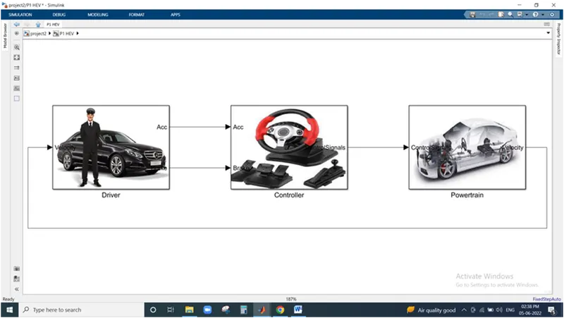
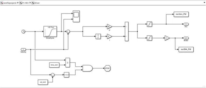
2].Driver:It is modeled using a ‘Driver’ block, which is a basic PI controller that generates accelerator and brake pedal outputs to match the desired and actual vehicle speeds. In this we use drive cycles fro the based on these results of fuel consumption and emissions the vehicle gets certified and it also forms a basis of uniform asessment. It is based on time, velocity then its all integrate and creates output accelration pedal and brake pedal.

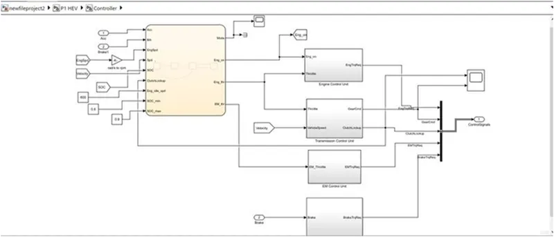
3] Controller:-The Controller block is the brains of the vehicle its representing the electronic controls units. It is based on the driver inputs, it generates desired engine torque, desired transmission gear desired motor torque and desired brake torque. These inputs are fed to the ‘Powertrain’ block which represents the drivetrain of the vehicle. In this we require to create stateflow block it explain in next figure.

4] Stateflow for Controller:-

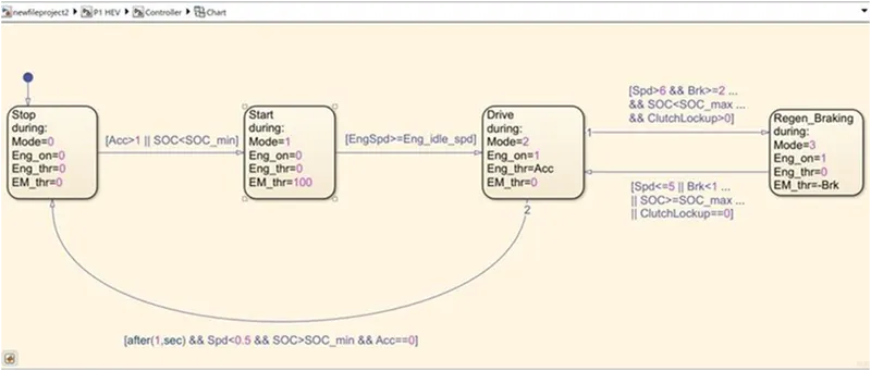
In this we created four conditions as stop, start, drive and regenration braking. The initial block represent the stop condition. In which the engine is off. The engine and motor throttle conditions are zero. Then the second block represent start condition. In which the mode is 1 the electric motor throttle is only used to provide the required torque and power to the vehicle. the engine is off and engine throttle conditionis zero.

The state 1 and state 2 are connected using the links i.e. it moves from state 1 to state 2 when acceleration is less than one or SOC is less then the minimum SOC.

State 3 Represtents mode 2 ii.e. engine is on and the engine throttle is also having positive value from the driver but the electric motor throttle is zero. It changes form state 2 to state 3 when engine speed is graeter than or equal to engine idle speed.

state 4 represents regenrative braking which is model 3 In this state the engine is on but the engine throttle is having no input from driver whereas the electric moto receives the negative power due to braking.

The inputs are given to chart is Acceleration, barke, engine speed, vehicle speed, SOC, and clutch lockup.

The output we get from the chart is mode, engine condition, engine throttle condition, and electric motor throttle condition.

Modification done in all Unit modeling. they showed in next figures.

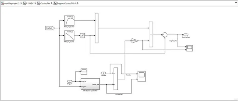
5] Engine Control Unit:-In this control model We use engine control unit in that give input Engine speed through creating look up table. in that table we give input Maximum torque and map speed then also create 2nd look up trable in that give input ct torque and map speed then it substracts and multiplied. the engine speed also give to ideal contro speed to integrate from this we meet output of engine required torque.

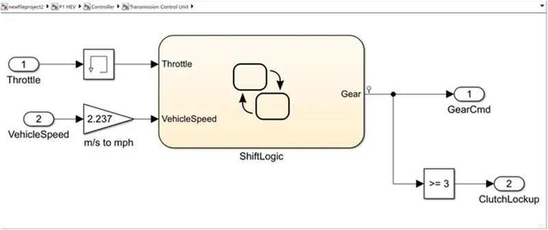
6] Transmission Control Unit:-In this unit we create steadfy flow variable state for controlling of gears of vehicle as in ascending and descending order with respect to time, speed, distance. and give input to this steady state is vehicle speed in m/s to mph.

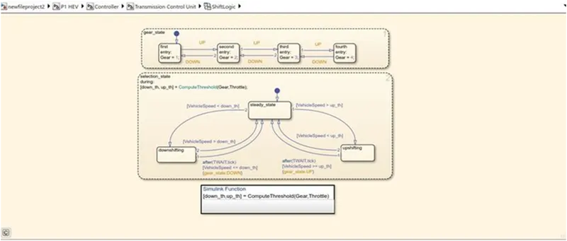
7] Shiftlogic:

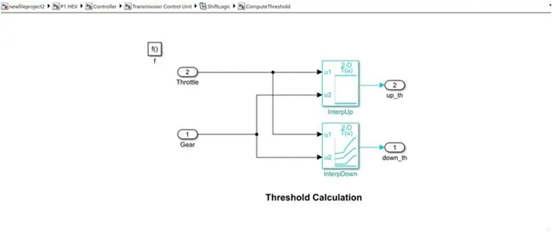
8] Threeshold Value in This controller:-

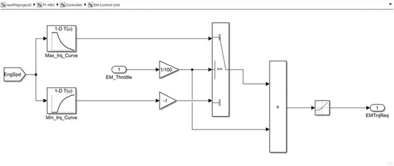
9] Electric Motor Control Unit:-

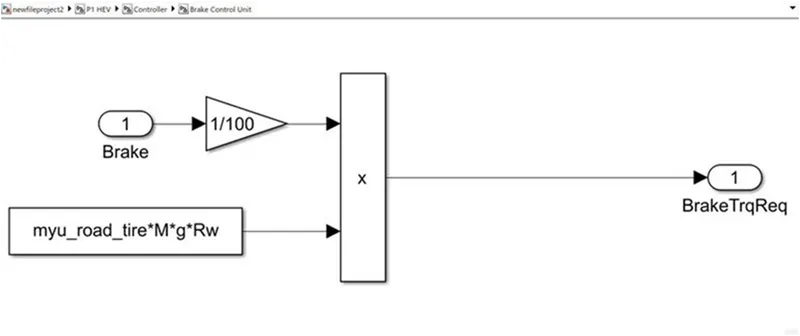
10] Brake Control Unit:-

In this calculate brake torque and then all three control signals output is give to powertrain.

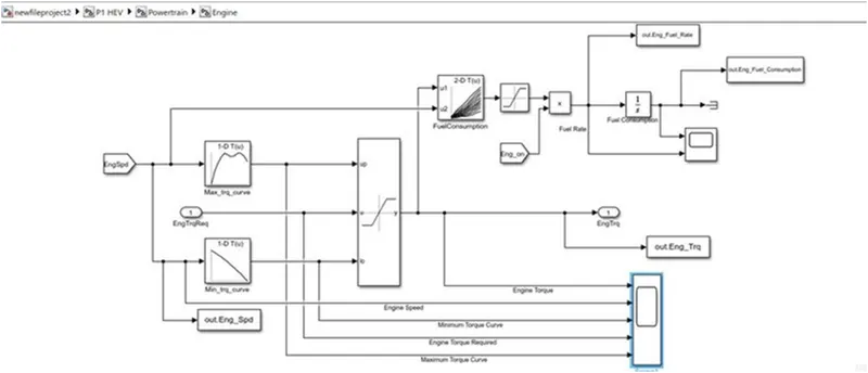
11] Engine:-In this model we used map based model to model the fuel consumption of engine. It is based on maximum Torque and minimum torque from the controller. and then it saturated torque and give output then saturated torque and speed map give fuel consumption takes the speed and torque then the output goes into saturated then its integrated.

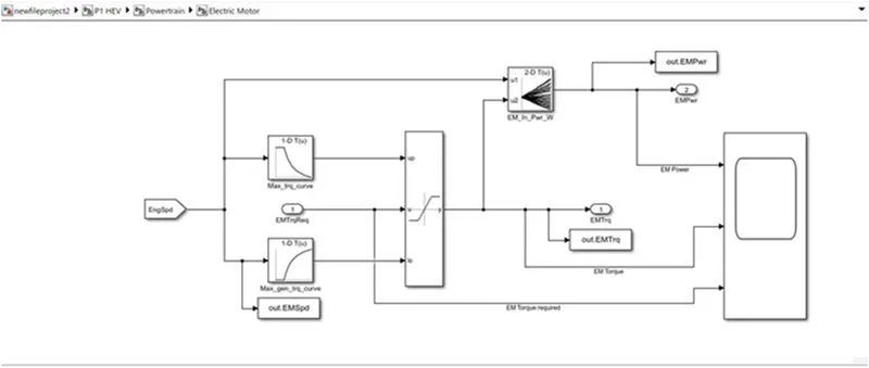
12] Electric Motor:-

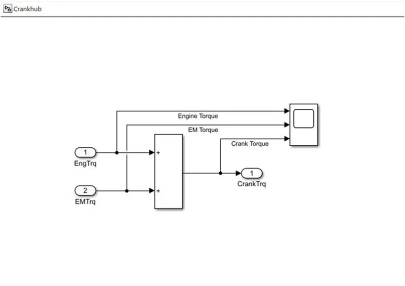
13] Crankhub:-

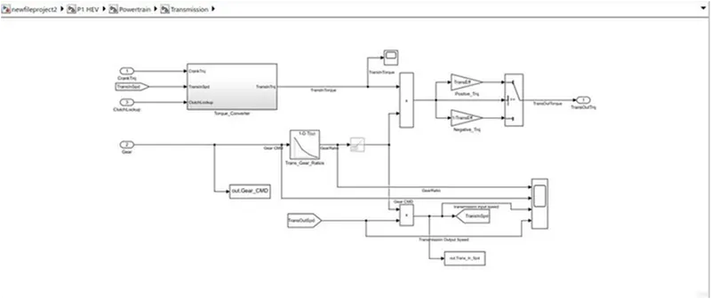
14] Transmission:-In these model we take engine torque, gear selector from controllerb for transmission of gear ratio. The ratio is multiply by transmission input torque and then the transmission efficiency positive torque and negative torque gives transmission input speed. In this case torque converter connects the engine to transmission it is part of transmission. In it basically engine dynamics and that is decoupled.

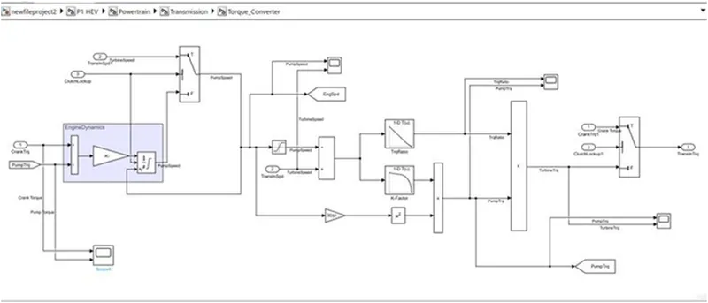
15] Torque Converter:-

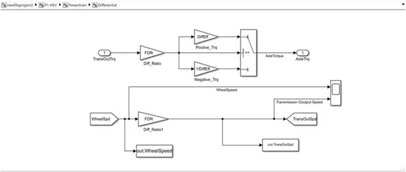
16] Differential:-In this taking input is the transmission output then its going to the differential ratio multiplied the output and input torque then meet axle torque. The axle torque is a lower than the transmission torque and differential ratio.

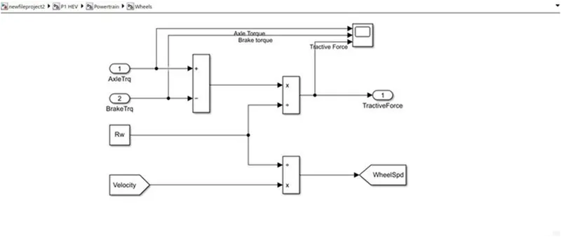
17] Wheel:-In this model we take the axle torque from differentail and brake torque from controller. it is substracts and multiplied rolling radius and velocity then we meet the tractive force from axle and brake torque. and the wheelspeed is meet using velocity.

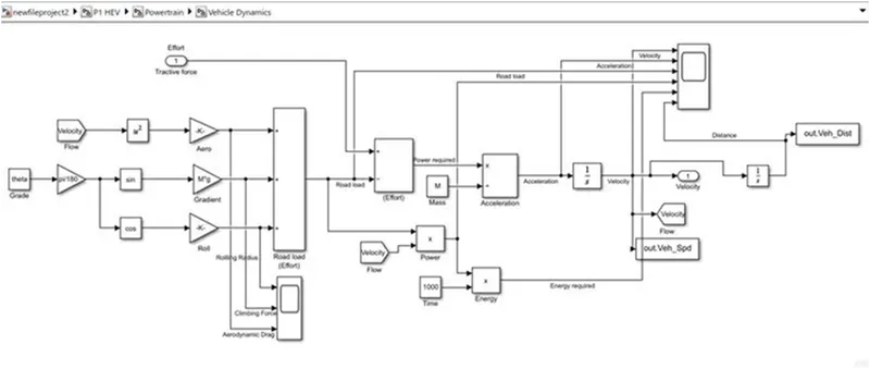
18] Vehicle Dynamics:-In this takes tractive force and road load. It is dictates vehicle speed based on tractive force and road load.

Battery Modeling:-

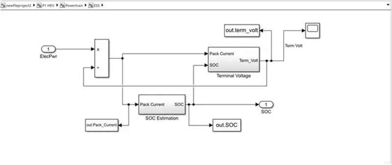
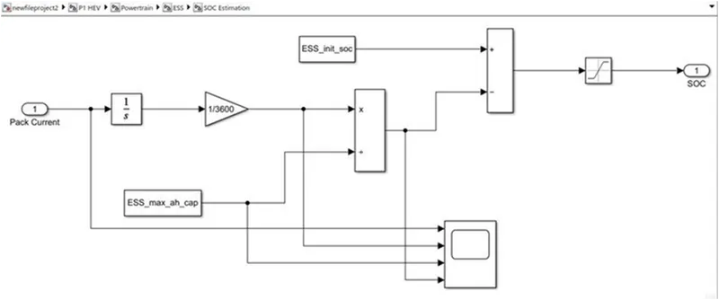
19] Estimated storage system:-In this we give input as power then it multiply and give to pack current. then from soc estimation meet output SOC its give to terminal voltage as input and then meet terminal voltage as output.

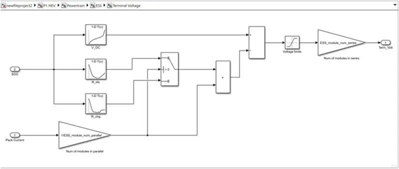
20] Terminal Voltage:-In this use input SOC it is connected to 1d lookup table 1st table variable interpolated as state of charge and open voltage circuit. In 2nd table variable interpolated as resistance discharge and state of charge and in 3rd table variable interpolated as resistance charge and state of charge. Then it is passed to switch block for controlling the threeshold. then they give voltage limits as max volts and min volts. then meet terminal Voltage.

21] Pack Current:-In this we integrate pack current and convert it rad to amp then saturated and meet SOC.

Then we create one coding file for creating plots and to meet all answers. that file shown in next.

Matlab code:

 
%% Renaming variables
Time = out.tout;
Acc_Pdl = out.Acc_Pdl;          % Accelerator pedal [%]
Brk_Pdl = out.Brk_Pdl;          % Brake pedal [%]
Gear_Cmd = out.Gear_CMD;        % Transmission gear
Trans_In_Spd = out.Trans_In_Spd*30/pi;  % Transmission input speed [rpm]
Trans_Out_Spd = out.TransOutSpd*30/pi;% Transmission output speed [rpm]
Eng_Trq = out.Eng_Trq;          % Engine brake torque [Nm]
Eng_Spd = out.Eng_Spd*30/pi;    % Engine speed [rpm]
Eng_Fuel_Consump = out.Eng_Fuel_Consumption;    % Engine fuel consumption [g]
Veh_Dist = out.Veh_Dist/1000;   % Distance traveled by vehicle [km]
Veh_Spd = out.Veh_Spd*18/5;     % Vehicle speed [kmph]
Wheel_Speed = out.WheelSpeed;     % Wheel speed [kmph]
Eng_Fuel_Rate = out.Eng_Fuel_Rate % Engine fuel rate [%]
EM_Speed = out.EMSpd*18/5;        % Electric Motor Speed
EM_Power = out.EMPwr;            % Electric Motor Power
EM_Torque = out.EMTrq;           % Electric Motor Torque
Term_Volt = out.term_volt;        % Terminal Voltage of battery
Soc = out.SOC;                    % State Of Charge
Pack_Current = out.Pack_Current;   %Pack current of battery
 
%% Data Analysis
Eng_Pwr = Eng_Spd*pi/30*Eng_Trq/1000;   % Engine brake power [kW]
rho_petrol = 0.7197;                    % Density of petrol [kg/L]
kmpl = Veh_Dist(end)/(Eng_Fuel_Consump(end)/1000/rho_petrol);    % Fuel economy [kmpl]
 
%% Plotting vehicle characteristics time trace to Engine speed, Engine Torque, Engine Power,
%  And Engine fuel rate, Engine fuel consumption
% Data conversion from Double Timeseries
 
Eng_spd = Eng_Spd.Data(:,1);   % engine speed
Eng_trq = Eng_Trq.Data(:,1);   % engine torque
Eng_pwr = Eng_Pwr.Data(:,1);   % engine power
Eng_fuel_rate = Eng_Fuel_Rate.Data(:,1);   % engine fuel rate
Eng_fuel_consumption = Eng_Fuel_Consump.Data(:,1);   % engine fuel consumption
EM_speed = EM_Speed.Data(:,1);   % motor speed
EM_power = EM_Power.Data(:,1);   % Motor Power
EM_torque = EM_Torque.Data(:,1);   % Motor Torque
Pack_current = Pack_Current.Data(:,1);  %pack current of battery
State_of_charge = Soc.Data(:,1);      %state of charge
Term_voltage = Term_Volt.Data(:,1);    % terminal Voltage of battery
 
%% Plotting vehicle characteristics time trace transmission IN/OUT and Wheel Speed
figure(1)
hold on
grid on
plot(Time, Trans_In_Spd, 'linewidth', 1, 'Color', 'black');
plot(Time, Trans_Out_Spd, 'linewidth', 1, 'Color', 'red');
plot(Time, Wheel_Speed, 'linewidth',1, 'color', 'blue')
ylabel('Speed [rpm]')
xlabel('Timem [s]')
xlim([0, Time(end)]);
ylim([0, 6000]);
legend('Trans Input','Trans Output','Wheel Speed');
 
%% Plotting Engine speed, Engine Torque, Engine Power,Engine fuel rate,Engine fuel consumption wrt Time
figure(2)
subplot(4,1,1)
plot(Time,Eng_trq,'linewidth',1,'color','black')
xlim([0, Time(end)]);
xlabel('Time [s]')
ylabel('Torque [Nm]')
legend('Engine Torque')
grid on
 
subplot(4,1,2)
plot(Time,Eng_pwr,'linewidth',1,'color','blue')
xlim([0, Time(end)]);
xlabel('Time [s]')
ylabel('Power [KW]')
legend('Engine Power')
grid on
 
subplot(4,1,3)
plot(Time,Eng_fuel_rate,'linewidth',1,'color','red')
xlim([0, Time(end)]);
xlabel('Time [s]')
ylabel('Fuel Rate [%]')
legend('Engine Fuel Rate')
grid on
 
subplot(4,1,4)
plot(Time,Eng_fuel_consumption,'linewidth',1,'color','green')
xlim([0, Time(end)]);
xlabel('Time [s]')
ylabel('Fuel Consumption')
legend('Engine Fuel Consumption')
grid on
 
% Plotting fuel economy Vs Engine Fuel consumption
figure(3)
plot(Eng_fuel_consumption,Eng_fuel_rate,'color','r')
xlabel('Fuel consumption')
ylabel('Fuel Rate [%]')
title('Fuel economy Vs Fuel Consumption')
grid on
 
%% Potting Accelerator pedal, Brake pedal and gear command with respect to time
figure(4)
subplot(2,1,1)
hold on
plot(Time, Acc_Pdl, 'linewidth', 1, 'Color', 'black');
plot(Time, Brk_Pdl, 'linewidth', 1, 'Color', 'red');
ylabel('Pedal [%]')
xlabel('Time [s]');
xlim([0, Time(end)]);
grid on
legend('Accel','Brake');
title('Acceleration & Brake Pedal wrt Time')
 
subplot(2,1,2)
plot(Time, Gear_Cmd, 'linewidth', 1, 'Color', 'black');
xlim([0, Time(end)]);
xlabel('Time [s]');
ylabel('Gear');
grid on
title('Gear command wrt Time')
 
% Plotting gear command vehicle desired with actual speed
figure(5)
subplot(2,1,1)
plot(Veh_spd, Gear_Cmd, 'linewidth', 1, 'Color', 'black');
xlabel('Speed [rpm]');
ylabel('Gear');
grid on
title('Gear command wrt vehicle speed')
 
subplot(2,1,2)
plot(Veh_dist, Gear_Cmd, 'linewidth', 1, 'Color', 'red');
xlabel('Distance [kmpl]');
ylabel('Gear');
grid on
title('Gear command wrt Distance')
 
%% Plotting engine operating points on engine fuel map
figure('Name','Engine Operating Points');
hold on
grid on
title('Engine Operating Points','fontsize',12);
p1=plot(Eng_map_spd*30/pi,Eng_max_trq,'linewidth',2,'color','r');
p2=line([Eng_map_spd(end)*30/pi Eng_map_spd(end)*30/pi],[0 Eng_max_trq(end)]);
set(p2,'linewidth',1,'linestyle','--','color','k');
p3=line([Eng_map_spd(1)*30/pi Eng_map_spd(1)*30/pi],[0 Eng_max_trq(1)]);
set(p3,'linewidth',1,'linestyle','--','color','k');
[c,h] = contour(Eng_map_spd'*30/pi,Eng_map_trq,Eng_fuel_map');
clabel(c,h);
xlabel('Engine Speed [rpm]');
ylabel('Engine Torque [Nm]');
title('Engine Fuel Consumption Map [g/s]');
legend([p1 p3],{'Max Curve','Operating Points'});
axis([Eng_map_spd(1)*30/pi Eng_map_spd(end)*30/pi 0 Eng_map_trq(end)]);
 
%% State of Charge, Pack Current, And Terminal Voltage with respect to Time
figure(6)
subplot(3,1,1)
plot(Time,Pack_current,'linewidth',1,'color','black')
xlim([0, Time(end)]);
xlabel('Time [s]')
ylabel('Current [W]')
legend('Pack Current')
grid on
 
subplot(3,1,2)
plot(Time,State_of_charge,'linewidth',1,'color','blue')
xlim([0, Time(end)]);
xlabel('Time [s]')
ylabel('Charging [%]')
legend('State Of Charge')
grid on
 
subplot(3,1,3)
plot(Time,Term_voltage,'linewidth',1,'color','red')
xlim([0, Time(end)]);
xlabel('Time [s]')
ylabel('Voltage [V]')
legend('Terminal Voltage')
grid on
 
%% Motor Speed, Torque, Motor input power with respect to Time
figure(7)
subplot(3,1,1)
plot(Time,EM_power,'linewidth',1,'color','black')
xlim([0, Time(end)]);
xlabel('Time [s]')
ylabel('Power [W]')
legend('Electric Motor Power ')
grid on
 
subplot(3,1,2)
plot(Time,EM_torque,'linewidth',1,'color','blue')
xlim([0, Time(end)]);
xlabel('Time [s]')
ylabel(' Torque [Nm]')
legend('Electric Motor Torque')
grid on
 
subplot(3,1,3)
plot(Time,EM_speed,'linewidth',1,'color','red')
xlim([0, Time(end)]);
xlabel('Time [s]')
ylabel('Speed [Rpm]')
legend('Electrical Motor Speed')
grid on
 
%% Plotting EM Operating Points on motor input power Map
figure('Name','Electric Motor Operating Points');
hold on
grid on
title('Electric Motor Operating Points','fontsize',12);
p1=plot(EM_map_spd*30/pi,EM_max_trq,'linewidth',2,'color','r');
p2=line([EM_map_spd(end)*30/pi EM_map_spd(end)*30/pi],[0 EM_max_trq(end)]);
set(p2,'linewidth',1,'linestyle','--','color','k');
p3=line([EM_map_spd(1)*30/pi EM_map_spd(1)*30/pi],[0 EM_max_trq(1)]);
set(p3,'linewidth',1,'linestyle','--','color','k');
[c,h] = contour(EM_map_spd'*30/pi,EM_map_trq,EM_inpwr_map');
clabel(c,h);
xlabel('Motor Speed [rpm]');
ylabel('Motor Torque [Nm]');
title('Motor Input Power Map [g/s]');
legend([p1 p3],{'Max Curve','Operating Points'});
axis([EM_map_spd(1)*30/pi EM_map_spd(end)*30/pi 0 EM_map_trq(end)]);

Que:- Tabulate the fuel economy numbers (kmpl) for UDDS and HWFET cycle. Compare these numbers with the baseline numbers for conventional vehicle model from Project 1.

Answer:-

Fuel Economy Numbers for project 2

S.No Drive cycle Fuel Economy Number (KMpl)

1 UDDS 15.0773

2 HWFET 17.1613

As we see the fuel economy is high in HWFET compared to UDDS. It is happen because in urban driving the vehicle encounters more traffic and it has to stop for fever distance and it consumes more fuel at the starting. In HWFET the vehicle encounters no traffic and it moves without use of too much braking so it will have more fuel economy number.

Comparing with fuel economy numbers for project 1

S.No Drive cycle Fuel Economy Number (KMpl)

1 UDDS 14.209

2 HWFET 16.503

As we see the fuel economy numbers for project 2 are little higher when compared to project 1,Deu to implementing the electric motor as it is P1 hybrid it may not have much variation in the fuel economy but as we implement other architechture it will increase by huge amount.

Que:- Plot the time trace for engine, transmission input, transmission output and wheel speed on one plot.

Answer:-

1] For UDDS drive cycle:-

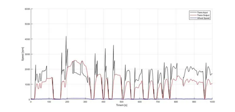
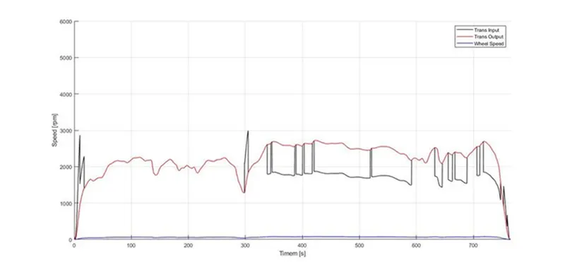
2] For HWFET drive cycle:-In this we can see the graph is more fluctuate into UDDS drive cycle compared to HWFET drive cycle. It is because UDDS has more starts and stops and in HWFET less starts and stops.

• Braking is high in UDDS compared to HWFET.
• Peaked engine power reached nearly 4200 RPM in UDDS drive cycle and in HWFET cycle it reached at 3000 RPM.

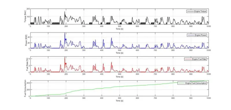
Que:- Plot engine torque, engine power, fuel rate and fuel consumption using subplots.

Answer:-

1] For UDDS drive cycle:-

2] For HWFET drive cycle:-

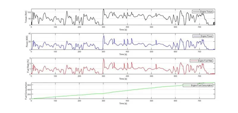
So we can conclude that Vehicle cosumed more power in UDDS drive cycle bacause in urban area the vehicle require many starts and stops so it required more power compred to HWFET.

In UDDS drive cycle Engine is high compred to HWFET drive cycle because the starting from rest the vehicle requires more torque to overcome the static friction.

The fuel rate is high in HWFET drive cycle compared to UDDS drive cycle because it will be in continues movement so it consumes more fuel.

The fuel economy is high in HWFET because In UDDS cycle many starts and stops so more fuel cosumes and the engine is in idle postion.

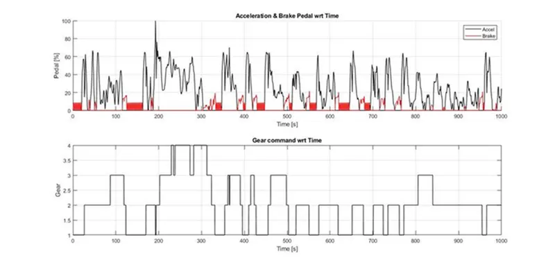
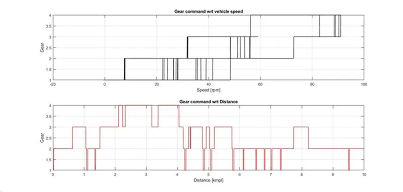
Que:- Plot accelerator and brake pedal, gear command, vehicle desired and actual speed, vehicle distance using subplots.

Answer:-Plot are shown are as follows.

1] For UDDS drive cycle:-

2] For HWFET drive cycle:-

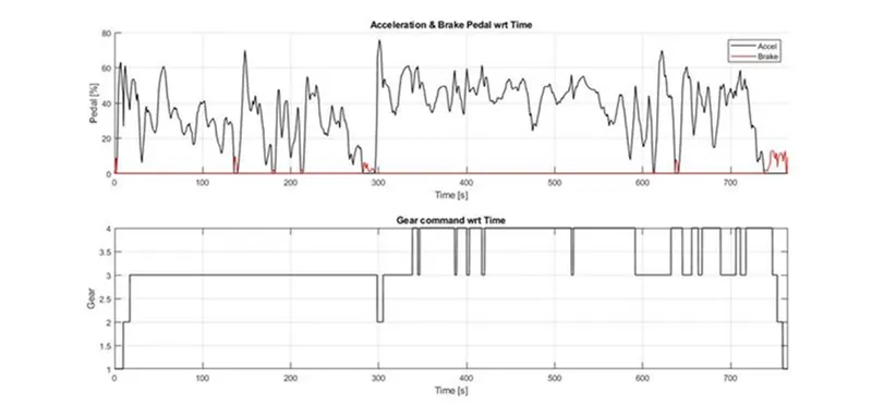
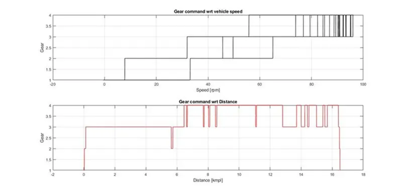
• In UDDS The acceleratior and brake pedal have more fluctuations because of frequently starts and stops. but in HWFET the brake pedal fluctuations are almost near to the zero line as there will be no frequent stops.
• In UDDS cycle mostly runs on 1st and 2nd gears and the 3rd and 4th gears are rarely useas it does not achieve high speed inn that traffic. In The HWFET cycle the vehicle mostly runn in 3rd and 4th gears as it will moving at high speeds.

Que:- Plot the engine operating points on the engine fuel map.

Answer:-

1] For UDDS drive cycle:-

2] For HWFET drive cycle:-

Que:- Plot motor speed, torque, motor input power using subplots.

Answer:-

1] For UDDS drive cycle:-

2] For HWFET drive cycle:-

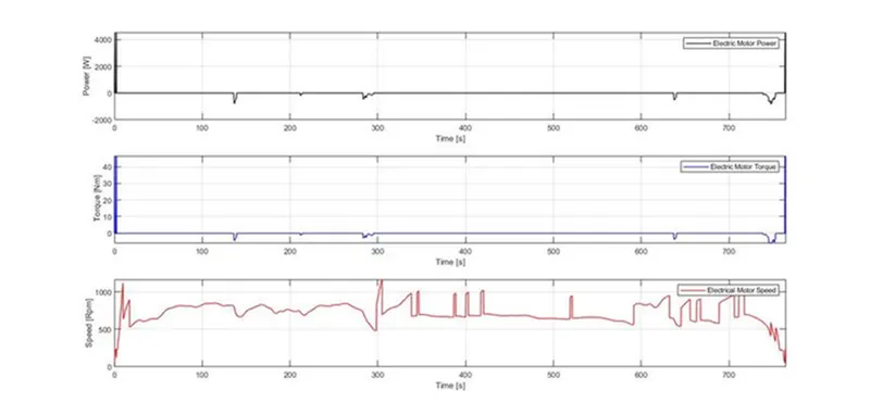
• The fluctuations will be more in UDDS cycle compared to HWFET cycle because UDDS has many starts and stops due to traffic as the purpose of motor in P! hybrid is initiation of crank rotation and they are more in UDDS cycle when compared to HWFET cycle.
• If the purpose of the motor is to provide traction then both the cycles wouldb have more flyctuations.
• So We can observe that the motor power and torque are very high in HWFET at the start and they are almost zero after few seconds but in UDDS it has contineud fluctuations and this is happen because of frequent braking in UDDS.

Que:- Plot pack voltage, current and SoC using subplots.

Answer:-

1] For UDDS drive cycle:-

2] For HWFET drive cycle:-

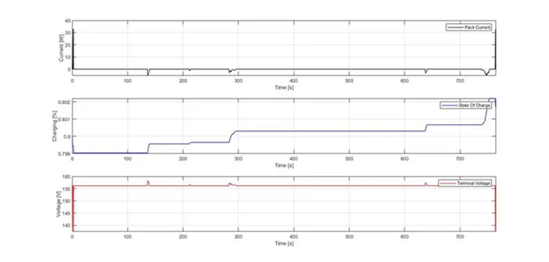
• The pack voltage and current will have more fluctuations in UDDS as compared to HWFET cycle because of the frequent start and stops throughout the drive and the battery has to provide the energgy everytime when the car is starting from the idle position.
• SOC decreased in the UDDS cycle wrt time but it has increased in HWFET cycle. It is because in UDDS we have frequent start and stops and battery has to provide the energy has evertytime when the caris starting from the idle position and the SOC decreases but in HWFET cycle The Vehicle will be moving continuously without braking frequently and the alternator is utilised to transfer some engine power to the battery through motor so SOC increase in the HWFET cycle.

Que:- Plot the motor operating points on the motor input power map, with the motor max motoring and generating torque curves.

Answer:-

1] For UDDS drive cycle:-

2] For HWFET drive cycle:-

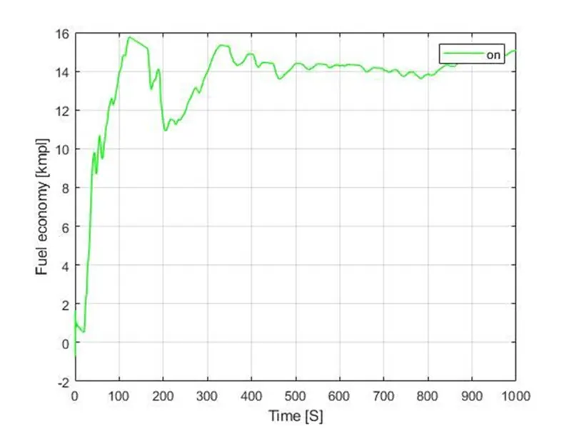
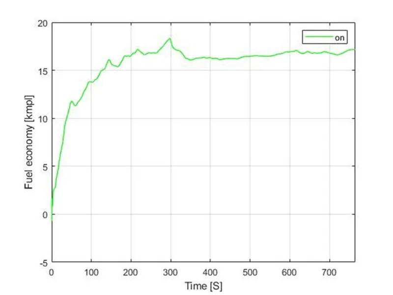
Fuel Economy wrt Time:-

1] For UDDS drive cycle:-

2] For HWFET drive cycle:-

Conclusion:-

The various performance of characteristics and operating points of UDDS drive cycle and HWFET drive cycle are analysed and the graphs are plotted

• Time trace for engine, Transmission input, Transmission output and wheelspeed with respect to time.
• Engine torque, Engine power, Fuel rate and Fuel consumption with respect to time.
• Accelerator and brake pedal, gear command and vehicle desired, actual speed, vehicle distance with respect to time.
• Engine operating points on the engine fuel map with respect to time.
• Motor speed, Torque, Motor input power with respect to time.
• Pack voltage, Current and State of charging with respect to time.
• The motor operating points on the motor input power map with respect to time.