Week 3 - Solving second order ODEs

AIM: To solve ordinary differential equattion(ode) and use the calculated information yo animate the motion of pendulumin Metalab.

Theory:Ordinary differential equation helps to solve the many engineering systems,such as harmonic motion,vibration,damping. it used to model many engineering systems.

Pendulum have many application and were utilized often before the digitl age.it used un clock and metronomes due to its regularity of their period.

the equation is given by:

its fundamental ODE function

where,

g = gravity in m/s2,

L = length of the pendulum in m,

m = mass of the ball in kg,

b=damping coefficient.

EXPLANATION: INPUTS are taken

L=1 metre,

m=1 kg,

b=0.05.

g=9.81 m/s2.

close all ,clear all, clc. all these command used for clearing all pre-existing data in command or workspacde window.

markersize- command use for form bob of pendulum and M command use for capture the current frame every time for loop run, the final step of loop is to add a+1 to the ct variale and ,end command use for plot and loop to stop both from running. and finnally to create movie ,movie command is used,videowriter command used for assign the video format for this project avi. used,open comand used for open the video, writevideo command used for write video and close command used for close the video file.

Initial condition: angular displement=0,angular velocity=5 rad/sec,time=0

solving ODE: ODE solver ode 45 is used in this program,ode_func is made for solve the given equation.

MATALAB CODE:

close all
clear all
clc
% solvig the second order ode and show animation
b=0.05;
l=1;
m=1;
g=9.81;
%initial codition
theta_0=[0;5];
%time points
t_span=linspace(0,20,500);

%solve ode
[t,results]= ode45(@(t,theta)ode_func(t,theta,b,g,l,m),t_span,theta_0);
figure(1)
plot(t,results(:,1))
hold on
plot(t,results(:,2))
xlabel('time')
ylabel('velocity')
legend('displacement','angular velocity')
grid on
hold off
displacement= results(:,1);
velocity=results(:,2);
%fixed coordinate
x0=1;
y0=1;
ct=1;
for i= 1:length(displacement)
    %coordinates
    x1=1-l*sin(displacement(i));
    y1=1-l*cos(displacement(i));
    figure(2)
    %plot fixed link
    plot([0 2],[1 1],'linewidth',15,'color','b')
    hold on
    plot([1 x1],[1 y1],[x1 x1],[y1 y1],'o','markersize',25,'color','r','linewidth',4)
    plot(x0,y0,'o','markersize',3,'color','green')
    %axis setting
    axis([0 2 -0.5 2])
    M(ct)=getframe(gcf);
    ct=ct+1;
    hold off
end
%making video file
movie(M)
videofile=VideoWriter('simple_pendulum.avi')
open(videofile)
writeVideo(videofile,M)
close(videofile)
function [dtheta_dt]=ode_func(t,theta,b,g,l,m)
theta1= theta(1);
theta2=theta(2);
dtheta1_dt=theta2
dtheta2_dt=(-(b/m)*theta2 -(g/l)*sin(theta1));
dtheta_dt=[dtheta1_dt;dtheta2_dt];
end

ERROR: no major error faced.

OUTPUT:

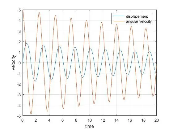
Animation video: Here is the link of animation of pendulum

https://youtu.be/5K_AOZuL_fA