Project 2 - Rankine cycle Simulator

Aim:To simulste a rankine cycle using matlab.

Objective:Exracting the Steam data and water properties from Xsteam data (IAPWS IF-97 standard)

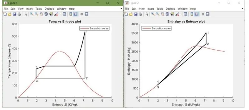
plotting the T vs s H vs s plot for given input

Rankine cycle:

Its thermodynamic cycle or heat engine in whoch fuel is used to produce heat with in boiler converting water into steam which then expand through turbine producing useful work .it is cycle which is converts the heat into mechanical energy which usually converted into electrical energy.

process and working:

process: 1-2: Isentropic Expansion in turbine

process:2-3:costant pressure heat rejection in condensor

process:3-4:Isentropic Compression in pump

process:4-1:costant pressure heat addition in boiler.

• Working of rankine cycle simulator.

1. in process 1-2: dry saturated vapoure expand through turbine and due to this decrease the presuure and temperature of vapoure and some condensation may occure.
2. process 2-3:vapore mixture leaving turbine is condensed at low pressure,in surface condensor using cooling water.In well design and maintained condensors pressure of vapore below from atomosperic pressure of operating fluid of cooling water temp.
3. process 3-4: now pressure of condenser is raised in the feed pump because of low specific volume of liquid
4. process4-1:high opresure liquid enters in boiler from feed pump and heated the saturation temp. further addition of energy causes evaporation of liquid until its fully convert into saturated steam.

Program:

clear all
close all
clc
file=fopen('XSteam data','r')
%displaying
disp('rankine cycle');
disp('1-2 is isentropic expansion in the turbine')
disp('2-3 is constant pressure heat removal in the condenser');
disp('3-4 is isentropic compression in the pump');
disp('4-1 is constant pressure heat  addition in the boiler');
% obtaining the input data
p1=input('nValue of pressure at turbine inlet p1')
T1=input('nValue of tempreature at turbine inlet T1')
p2=input('nValue of temprature at condenser inlet p2')
%extracting data_defining variables
%state 1
h1=XSteam('h_pt',p1,T1);
s1=XSteam('s_pt',p1,T1);
% state 2
s2=s1;
sf2=XSteam('sL_p',p2);
sg2=XSteam('sV_p',p2);
x2=(s2-sf2)/(sg2-sf2);
hf2=XSteam('hL_p',p2);
hg2=XSteam('hV_p',p2);
h2=hf2 + (x2*(hg2-hf2));
%state 3
p3=p2
s3=XSteam('sL_p',p3);
h3=XSteam('hL_p',p3);
%state 4
s4=s3
p4=p1
%work done by turbine
wt=h1-h2;
%work done to run pump
v3=XSteam('vL_p',p3);
wp=v3*(p4-p3)*100;
h4=h3 + wp;
%net work
wnet=wt - wp;
%heat into system
Qin=h1-h4
%heat out of system
Qout=h2-h3
%thermal efficiency
eff=(wnet/Qin)*100;
%Specific Steam consumption
%SSC= mass flow rate/power
SSC=(3600/wnet)

%calculating temperature at state point
T3= XSteam('Tsat_p',p3);
T2=T3;
Cp4=XSteam('Cp_ps',p4,s4);
Cv4=XSteam('Cv_ps',p4,s4);
k=Cp4/Cv4;
T4=T3/((p3/p4)^((k-1)/k));
%calculating temp.,entropy,enthalpy  at vapoure and liquid line
%line fpor plotting
T6=XSteam('Tsat_p',p1);
s5=XSteam('sL_p',p1);
s6=XSteam('sV_p',p1);
h5=XSteam('hL_p',p1);
h6=XSteam('hV_p',p1);
T5=T6;
%plotting the saturation  curve
T= linspace(1,375,1000);
for i=1:length(T)
    sf(i)=XSteam('sL_T',T(i));
    sg(i)=XSteam('sV_T',T(i));
    hf(i)=XSteam('hL_T',T(i));
    hg(i)=XSteam('hV_T',T(i));
end
%ploting T-S diagram
figure(1)
hold on
plot(sf,T,'r','linewidth',1)
plot(sg,T,'r','linewidth',1)
plot([s1 s2],[T1 T2],'k','linewidth',2)
plot([s2 s3],[T2 T3],'k','linewidth',2)
plot([s3 s4],[T3 T4],'k','linewidth',2)
plot([s4 s5],[T4 T5],'k','linewidth',2)
plot([s5 s6],[T5 T6],'k','linewidth',2)
sc1= linspace(s6,s1,1000);
for l=1:length(sc1)
    Tc1(1)= XSteam('T_ps', p1,sc1(l));
end
plot(sc1.Tc,'k','linewidth',2)
text(s1+0.1,T1,'1')
text(s2+0.1,T2,'2')
text(s3,T3-20,'3')
text(s4,T4+20,'4')
title('temp vs Entropy plot')
xlabel('Entropy ,S(kj/kgk')
ylabel('Temperature')
legend('saturation curve')
%plotting h-s digram
figure(2)
hold on
plots(sf,h,'r','linewidth',1)
plot(sg,hg,'r','linewidth',1)
plot([s1, s2],[h1 h2],'k','linewidth',2)
plot([s2, s3],[h2 h3],'k','linewidth',2)
plot([s3, s4],[h3 h4],'k','linewidth',2)
hc=linspace(h4,h5,100);
for k=1:length(hc)
    sch(k)=XSteam('s_ph',p1,hc(k));
end
plot(sch,hc,'k','linewidth',2)
plot([s5s 6],[h5 h6],'k','linewidth',2)
for m=1:length(sc1)
    hc1(m)=XSteam('h_ps',p,sc1(m));
end
plot(sc1,hc1,'k','linewidth',2)
text(s1+0.1,h1,'1')
text(s2+0.1,h2,'2')
text(s3,h3-100,'3')
text(s4,h4+200,'4')
title('Enthalpy vs Entropy plot')
xlabel('Entropy')
yabel('Enthalpy')
legend('saturation curve','locaton','northwest')
%Displyaing results
disp('RESULTS')
fprintf('At State point 1:n');
fprintf('p1: %8.3f barn',p1);
fprintf('T1: %8.3f Cn',T1);
fprintf('h1: %8.3f kj/kgn',h1);
fprintf('s1: %8.3f kj/kgknn',s1);
fprintf('At State point 2:n');
fprintf('p2: %8.3f barn',p2);
fprintf('T2: %8.3f Cn',T2);
fprintf('h2: %8.3f kj/kgn',h2);
fprintf('s2: %8.3f kj/kgknn',s2);
fprintf('x2: %8.3fnn',x2);
fprintf('At State point 3:n');
fprintf('p3: %8.3f barn',p3);
fprintf('T3: %8.3f Cn',T3);
fprintf('h3: %8.3f kj/kgn',h3);
fprintf('s3: %8.3f kj/kgknn',s3);
fprintf('At State point 4:n');
fprintf('p4: %8.3f barn',p4);
fprintf('T4: %8.3f Cn',T4);
fprintf('h4: %8.3f kj/kgn',h4);
fprintf('s4: %8.3f kj/kgknn',s4);
fprintf('Trbine work: %8.3f kj/kgn',wt);
fprintf('pump work: %8.3f kj/kgn',wp);
fprintf('wnet: %8.3f kj/kgn',wnet);
fprintf('efficiency: %8.3f percent n',eff);
fprintf('S.S.C: %8.3f kj/kwh',SSC);

code Explanation:

• Xsteam data is used to extract steam and water properties of enthalpy,entropy,sp.presssure and temp. for sat. liqiud sat. vapoure condition etc.
• programme required input of pressurein bar at state point 1 (turbine inlet),temp. at same point and temp. incondensor inlet(point 2)
• with the help of this input and from Xsteam data we cancalculate all state point of the rankine cycle
• The Xsteam data works as

h1=Xsteam('h_pt',p1,T1):(return the enthalpy of water at given pressure and temp. )

• we extract the data ,we use thermodynamic relation to further find state point and extract their datafrom Xstraem.
• Sf and Sg,hf and hg where f and g standa on saturated liquid and saturated vapoure respectively.
• The net work done by turbine,work done to run the pump,heat in and heat out are calculated using standard thermodynamic relation
• T,s h are calculated at vapoure and liquid line plotting purpose
• saturation curve is plotted in red for saturated liquid and saturated gas
• plot T vs s and h vs s is created from all line obtainedfrom the program.
• the plot changes as user input changes PLOT:
• T vs S and H vs S
•