Week 4.1 - Genetic Algorithm

AIM:

• To study about genetic algorithm and calculate the global maxima of stalagmit function using Genetic Algorithm in matalab.

OBJECTIVE:

• To study about genetic algorithm andstalagmite function
• to Write a code in MATLAB to optimise the stalagmite function and find the global maxima of the function.
• To plot graph on baiss of sudy for genetic algorithm

INTRODUCTION:

A genetic algorithm (ga ) is use for solving both constraind and unconstrined optimization problem based on natural selection process that mimics biological evolution.We can apply GA to solve problem that are not well suited for standadt optimisation algorithms by default in Metalab ,GA calculates the minimum value of function ,so to find global maximum of function we can invert the function whose global maximum is to befound,find the minimum value of the inverted function so negative of inverted value is give the global maximum of function.

EXPLANATION:

primary stage is to create function to calculate the value of objective function at various value of x and y .we use linspace command ,then we creatematrix using meshgrid function ,now value in different matrix created can be put as an input into function that we have created by calling it, then we need to calculate maximum value which is calculated by GA and its inbuild function.So we use the loop and iterate it 50 times.

command:

surf : use for create surface to visualise the function.

marker:to find point of local maximum.

tic, toc: used for look at time taken for evaluatin

Syntax for defining 'ga' in matalab:

• x=ga(fun,nvars)

where, x=optimal variable, fun=objective function, nvras=number of variable, but sometime[x,fval] is used insted of 'x' where'fval' gives objective function.

• x=ga(fun,nvras,A,B,Aeq,Beq,lb,ub)

where,

A,B=liniear inequation constraints

Aeq,Beq=liniear equality constraints

it there are no liniear equlities and inequality then A,B,Aeq,Beq are set to'[]'

x=ga(fun,nvras,A,B,Aeq,Beq,lb,ub,nonlcon,intcon,option)

where,

nonlcon= nonlinier constrints,lb=lower bound,ub=upper bound.

intCon=integer values

options=optimization option

if there are non linear constrints and integer value the noncolon and intColon are set to'[]'.

clear all
close all
clc
%definig the search space
x=linspace(0,0.6,150);
y=linspace(0,0.6,150);
%matrix
[xx,yy]=meshgrid(x,y)
%number of iterations
n=50;
%starting thre loop
for i=1:length(xx)
    for j=1:length(yy)
        input_vector(1)=xx(i,j);
        input_vector(2)=yy(i,j);
        f(i,j)=stalagmite(input_vector);
    end
end

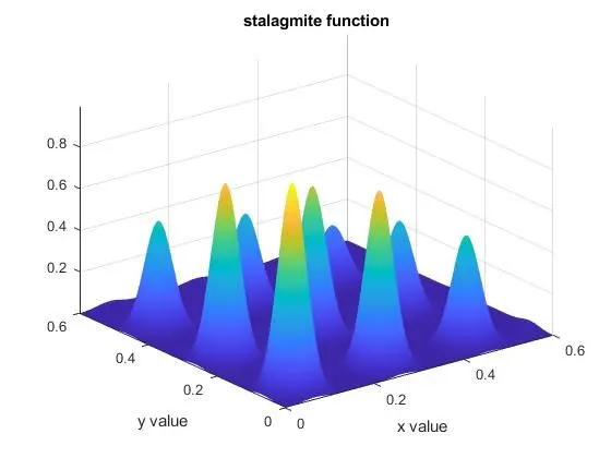
%create three dimensional surface

surfc(xx,yy,-f)
shading interp
xlabel('x value')
ylabel('y value')
title ('stalagmite function')
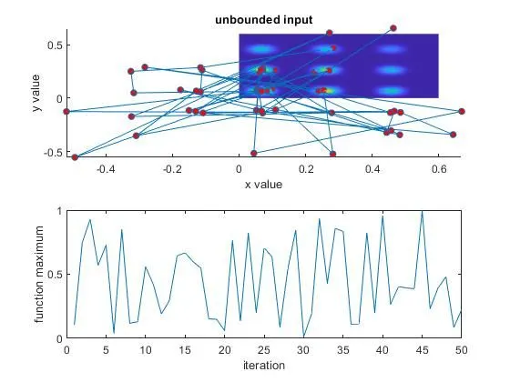
%study 1
tic
for i=1:n
    [inputs,fopt(i)]=ga(@stalagmite,2);
    xopt(i)=inputs(1);
    yopt(i)=inputs(2);
end
study_1=toc
figure(2)
subplot(2,1,1)
hold on
surfc(x,y,-f)
title('unbounded input')
xlabel('x value')
ylabel('y value')
shading interp
hold on
plot3(xopt,yopt,-fopt,'marker','o','markersize',5,'markerfacecolor','r')
subplot(2,1,2)
plot(-fopt)
xlabel('iteration')
ylabel('function maximum')
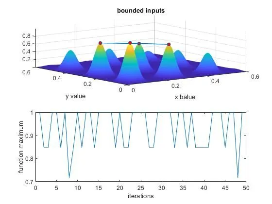
% case 2nd wih upper and lower bounds
tic;
for i=1:n
    [inputs,fopt(i)]=ga(@stalagmite,2,[],[],[],[],[0;0],[0.6;0.6]);
    xopt(i)=inputs(1)
    yopt(i)=inputs(2)
end
study_2_time=toc
figure(3)
subplot(2,1,1)
surfc(x,y,-f)
shading interp
title('bounded inputs')
xlabel('x balue')
ylabel('y value')
hold on
plot3(xopt,yopt,-fopt,'marker','o','markersize',5,'markerfacecolor','r')
subplot(2,1,2)
plot(-fopt)
xlabel('iterations')
ylabel('function maximum')
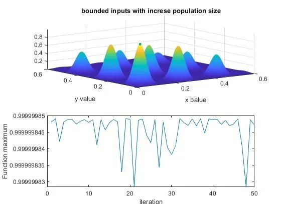
% study3 increasing the population size
% by doing sowe are incfreasing the probability of function
% to converge at global maximum
options=optimoptions(@ga)
options=optimoptions(@ga,'populationsize',500)
tic
for i=1:n
    [inputs,fopt(i)]=ga(@stalagmite,2,[],[],[],[],[0;0],[0.6;0.6],[],[],options);
    xopt(i)=inputs(1);
    yopt(i)=inputs(2);
end
study_3_time=toc
figure(4)
subplot(2,1,1)
surfc(x,y,-f)
shading interp
title('bounded inputs with increse population size')
xlabel('x balue')
ylabel('y value')
hold on
plot3(xopt,yopt,-fopt,'marker','o','MarkerSize',3,'MarkerFaceColor','green')
subplot(2,1,2)
plot(-fopt)
xlabel('iteration')
ylabel('Function maximum')
function [f]= stalagmite(input_vector)
a=input_vector(1);
b=input_vector(2);
term1=(sin((5.1*pi*a)+0.5))^6;
term2=exp(-4*log(2)*((a-0.0667)^2)/0.64);
term3=(sin((5.1*pi*b)+0.5))^6;
term4=exp((-4)*log(2)*((b-0.0667)^2)/0.64);
[f]=-(term1*term2*term3*term4);
end

• the -ve sign in function will invert the stalagmite plot which will give the function maxima.

OUTPUT: