Project 2

Aim :

To develop a forward energy based fuel consumption model of a P1 Hybrid electric vehicle in MATLAB and simulink.

Objective :

• Understand the concept of forward energy based fuel consumption model of a P1 Hybrid electric vehicle.
• To understand the functioning various vehicle components including engine, electric motor, battery ,torque converter, transmission system, longitudinal dynamics etc.
• Development of a Matlab script used to load all the variables required for running the simulink model.
• Development of a simulink model of the vehicle.
• Development of a MATLAB script to do some basic post-process calculations and generate results and plots.
• Analyzing the results.

Theory :

Hybrid Electric Vehicle - P1 Type

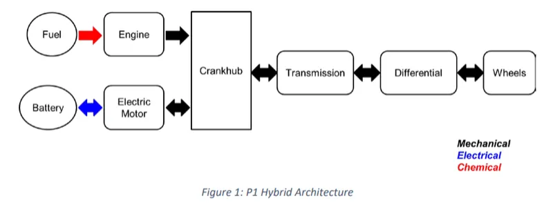
This P1 architecture, with the electric machine connected directly to the crankshaft, is the solution adopted by Honda on their first generation Integrated Motor Assist technology. The electric motor functions as a generator, during vehicle deceleration, as an engine starter, and as a motor to assist the engine during vehicle acceleration. One of the biggest advantage of this solution is that the electric motor can provide higher torque than the BiSG, since there is no belt limitation due to slip. However, since there is no speed/torque requirements on the electric motor can be quite demanding.

For, Examples of P1 MHEV architecture are.

1. Honda Insight Hybrid 2009 (with integrated Motor Assist technology)
2. Mercedes Benz S400 Bluehybrid 2010

Forward-Facing vehicle simulation :

One dimensional powertrain simulation used for a dynamic concept assessment and controller development. This simulation principle is commonly referred to as forward-facing simulation as shown in figure. A drive cycle in terms of vehicle speed is often used as a reference for a driver model to track. For on-road vehicles the load model is usually in terms of a fixed vehicle mass subjected to gravitational forces, areodynamic drag and rolling resistance. A driver model can in its simplest form be a simple P1 controller tracking a speed reference. For off road working machines with additional power consumers, the load and operator can be much more complex to model.

MATLAB initializing Code :

In this hybrid electric vehicle forward model use Honda Insight motor and battery are concidered for this project. Data is taken from ADVISOR data base developed by NREL, USA.

A MATLAB script "Project2_initFile.m" is to load the variable to the workspace that is to be used for further calculation/processing for the simulink model. A Honda Insight motor with the 10kW PMSM motor and 6Ah 154V NiMH battery pack. Transmission shift map and controller is taken from simulink exaple data base.

%%%%%%%%%%%%%%%%%%%%%%%%%%%%%%%%%%%%%%%%%%%%%%%%%%%%%%%%%%%%%%%%%%%%%
%% Skill-Lync -> Hybrid Drives Development
% Project 1 - Hybrid Vehicle Model
% By - Kaviyarasan K 

% Description:

%% Initialization File
% Initialization file for loading the variables for the Hybrid vehicle simulation model
close all
clear all
clc

%% Vehicle Parameters
M = 1500;       % Vehicle weight [kg]
Cr = 0.015;     % Rolling resistance coefficient
Rw = 0.35;      % Rolling radius [m]
Cd = 0.33;      % Drag coefficient
Af = 2;         % Frontal area [m2]
rhoa = 1.225;   % Air density [kg/m3]
Vwind = 0;      % Wind velocity [kmph]
g = 9.81;       % Gravitational acceleration [m/s2]
theta = 0;      % Slope [deg]
myu_road_tire = 1; % Coefficient of friction between tire - road interface

%% Powertrain Parameters 
FDR = 3.73;                         % Final Drive Ratio / Diff Ratio
DiffEff = 0.99;                     % Differential efficiency (assumed independent of operating conditions)

NumGear = 4;                        % Number of gears in transmission
TransGear = [1:NumGear];            % Transmission Gears
TransRatio = [3.06, 1.62, 1, 0.7];  % Corresponding Transmission ratios
TransEff = 0.90;                    % Transmission efficiency (assumed independent of operating conditions)

TC_SR = [0, .5, .6, .7, .8, .87, .92, .94, .96, .97, 1];   % Torque Converter Speed Ratio (Matlab default) -> TurbSpd/PumpSpd  
TC_TR = [2.232, 1.5462, 1.4058, 1.2746, 1.1528, 1.0732, 1.0192, 1, 1, 1, 1];   % Torque Converter Torque Ratio (Matlab default) -> TurbTrq/PumpTrq
TC_Cf = 1e-4 * [.72558, .66322, .63463, .59042, .51331, .4144, .29287, .22444, .12186, .04386, 0]; % Torque Converter Capacity Factor (Matlab default) -> PumpTrq/PumpSpd^2 [Nm/rpm^2]

load Vehicle_Data/Engine_data_1_9L_Saturn_95kW
load Vehicle_Data/Trans_Shift_map
load Vehicle_Data/EM_Honda_Insight_10kW
load Vehicle_Data/ESS_NiMH6


ESS_init_soc = 0.8;
ESS_soc_max = 0.9;
ESS_soc_min = 0.6;


%% Driver Parameters
Kp = 10;                    % P gain for driver PI model
Ki = 1;                     % I gain for driver PI model
Drive_Cycle_Select = 2;     % Drive cycle selection

%% Inputting the desired DriveCycle
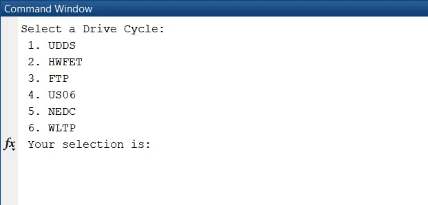
Drive_Cycle_Select = input(sprintf('Select a Drive Cycle: \n 1. UDDS \n 2. HWFET \n 3. FTP \n 4. US06 \n 5. NEDC \n 6. WLTP \n Your selection is: '));
% Drive cycle values in m/s

% Loading Drive Cycle values. Variables: cyc_time, cyc_vel
if Drive_Cycle_Select == 1
    load DriveCycles/UDDS;
    
elseif Drive_Cycle_Select == 2
    load DriveCycles/HWFET;
    
elseif Drive_Cycle_Select == 3
    load DriveCycles/FTP;
    
elseif Drive_Cycle_Select == 4
    load DriveCycles/US06;
    
elseif Drive_Cycle_Select == 5
    load DriveCycles/NEDC;
    
elseif Drive_Cycle_Select == 6
    load DriveCycles/WLTP;
 
end

time_end = cyc_time(end);
vel_end = cyc_vel(end);

%% Running Simulink Model 
%sim('Project2_VehicleModel');   % Run Simulink model

This code is designed such a way that it asks for the drive cycle that need to be used for the study and the user input decides the desired drive cycle for the study. The screenshot of the command window asking for the drive cycle of study is shown in figure. For the chosen drive cycle the simulink vehicle model will be run automatically, and after that MATLAB post processing script will be run automaticallly for providing the necessary plots for the study.

Simulink vehicle modlel :

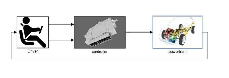
The simulink model consist of three main subsystem are Driver, controller, powertrain as shown in figure. The Driver subsystem generates the accelerator and brake pedal outputs to match the desired and actual vehicle speed. The controller block repersents the electrinic control units, which genarates the desired engine torque, desired transmission gear, desired motor torque and desired brake torque based on the driver inputs. The powertrain subsystem represents the actual vehicle consisting of all vehicle components which inputs the control signal from controller and provides actual vehicle motion charecteristics.

Driver Block :

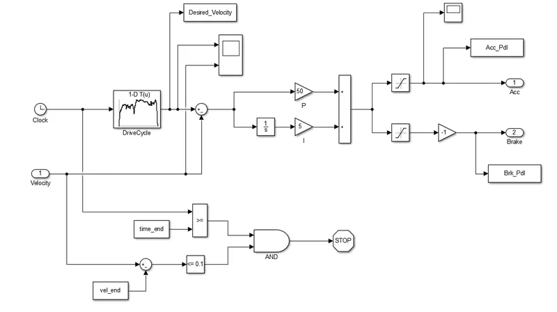
This block is basically a PI controller. A PI controller is a feedback control loop that calculates an error signal by taking the difference between the output of a system. It multiplies the error with constant gain for P nd I it integrates and them multiply with a smaller gain. The constant value for P and I are found by trial and error method. Here the error is the difference between the desired vehicle speed and the actual vehicle speed.

The saturation block extracts the positive and positive and negative signal as the acceleration pedal is passed on between the values 0 and 100 while for the brake pedal, the values between 100 and 0 are extracted. The comparative block compares the actual time and end time of drive cycle, similarly the current velocity is compared with the end velocity.

Controller Block :

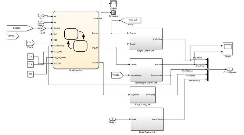
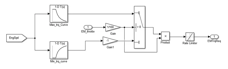
The output of the driver block which is the acceleration and brake pedal signal is passed on to the controller block. The controller block consist of four control unit are Engine control unit, Transmission control unit, EM control unit and Brake control unit. All these data from the four control unit goes to the bus creator. The bus creator is used to combine all these three signals to a one signal. This combined signal is then sent to the powertrain block.

Stateflow for Controller :

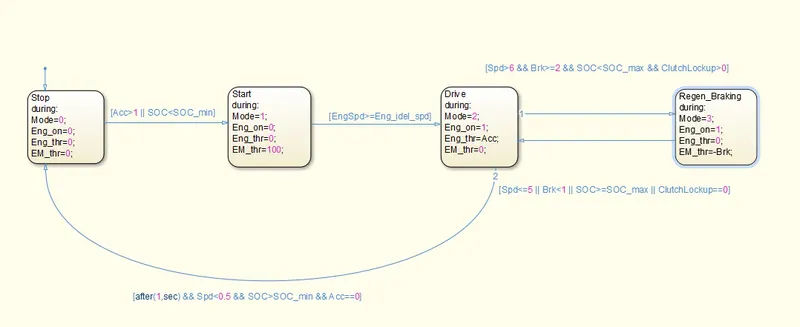
In this we created four conditions as stop, start, drive and regeneration braking. The initial block represent the stop condition. In which the engine is OFF. The engine and motor throttle conditions are zero. Then the second block represent start condition. In which the mode is 1 the electric motor throttle is only used to provide the required torque and power to the vehicle the engine is off and engine throttle conditions zero.

The state 1 and state 2 are connected using the links so, it moves from state 1 to state 2 when acceleration is less than one or SOC is less then the minimum SOC. State 3 represtents mode 2 so engine is on and the engine throttle is also having positive value from the driver but the electric motor throattle is zero. It changes from state 2 to state 3 when engine speed is grater than or equal to engine idle speed. state 4 represents regenerative braking.

Engine Control Unit :

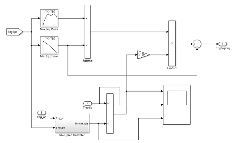
In this control model we use engine control unit in that give input engine speed through creating lookup table in that table we give input Maximum torque and map speed then also create 2nd lookup table in that give input ct torque and map speed then it substracts and multiplied. the engine speed also give to ideal control speed to integrate from this we meet output of engine required torque.

Idle speed controller :

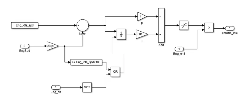
The idle speed controller is a PI controller where the engine speed and the idle speed of the engine is compared. The error is then multiplied with constant P and the integrated error is multiplied with constant 1.

Transmission Control Unit :

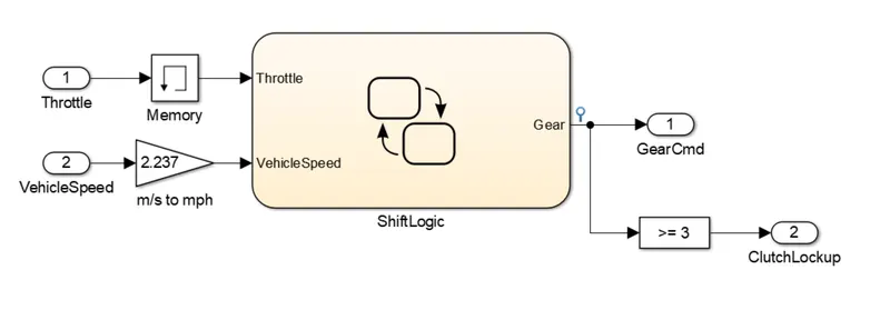
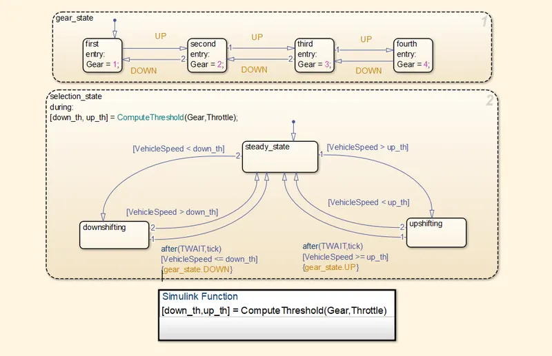
In this unit we create steady flow variable state for controlling of gears of vehicle as in ascenging and descending order with respect to time, speed, distance and give input to this steady state is vehicle speed in m/s to mph.

Gear shift logic unit :

Electrical control unit :

Brake control unit :

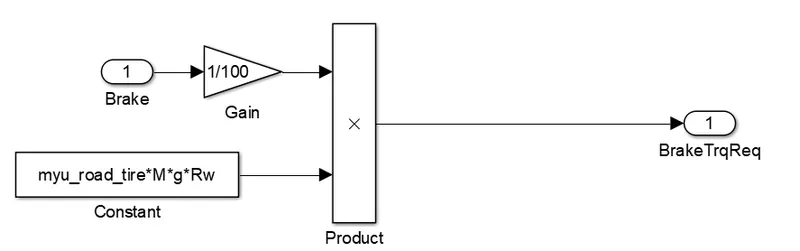
The Brake pedal signal from the driver block is multiplied with the maximum friction, which gives the maximum braking torque. The gain block is used convert to actual value from the percentage.

Powertrain :

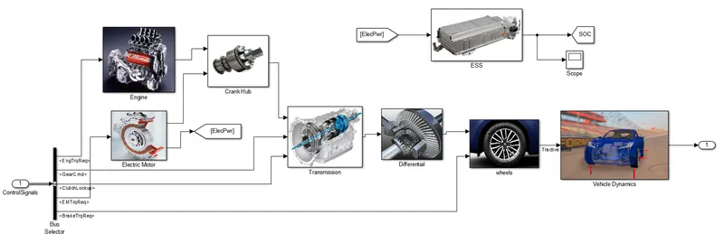
The powertrain block consist of several main subsystems are Engine, electrical motor, Crank hub, transmission, Differential, wheels, vehicle dynamics. The signal from the controller block are extracted using the bus selector, which consist of the signal for Engine torque requirement, Gear command and brake torque requirement.

Engine :

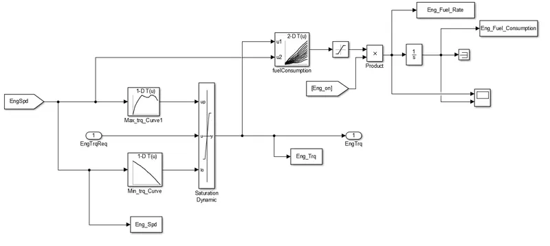
In this model we used map based model to model the fuel consumption of engine. It is based on maximum torque and minimum torque from the controller. And then it saturated torque and give output then satureted torque and speed map give fuel consumption takes the speed and torque then the output goes into saturated then its integrated.

Eletric Motor :

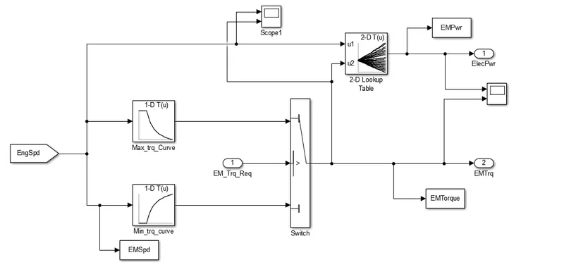
In this electric motor it get the engine speed as the input and it goes to the torque convertor. so it get the final motor torque and this torque is used to find the electric motor power by this torque and the speed of the motor as the inputs to thr 2D lookup table which is created by the power map has the torque data and the speed data for this it gives the corresponding electrical power as the output.

Crank Hub :

Transmission :

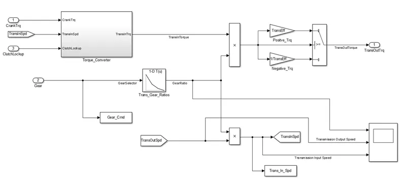
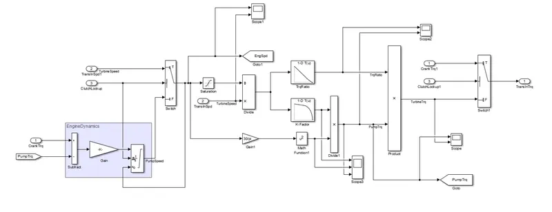
In this model we take engine torque, gear selector from controller for transmission of gear ratio. The ratio is multiply by transmission input torque and then the transmission efficiency positive torque and negative torque gives transmission input speed. In this case torque converter connects the engine to transmission it is part of transmission. In it basically engine dynamics and that is decoupled.

Torque Convertor :

Differential :

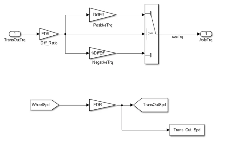
The Differential subsystem takes the output from the transmission system and reduce it as the gear ratio of the differential. The switch block is used to compensate for the negative and positive sign values. The required parameters are transferred between the other subsystem and the command window using the goto and to workspace blocks.

Wheels :

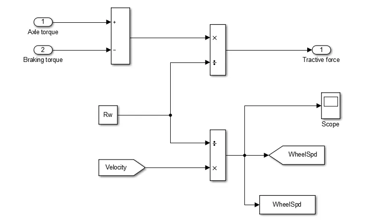
The wheels subsystem takes the axle torque and brake torque as the input. The brake torque is to reduce the axle torque to maintain the desired vehicle speed. Dividing the dynamic radius of the wheel with equivalent torque and vehicle velocity gives the tractive force and the wheel speed.

Vehicle Dynamics :

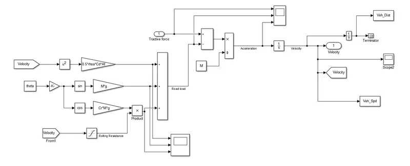
The vehicle dynamics block is used to find the vehicle dynamic characteristics like velocity, acceleration and distance travelled from the tractive force. The vehicle force corresponding to the actual vehicle is the difference between the tractive and the road load. The road load constitutes the drag, rolling and grading resistance. The velocity saturation is multiplied with the rolling resistance to ensure that it is avoided when the vehicle is not in motion.

Battery unit :

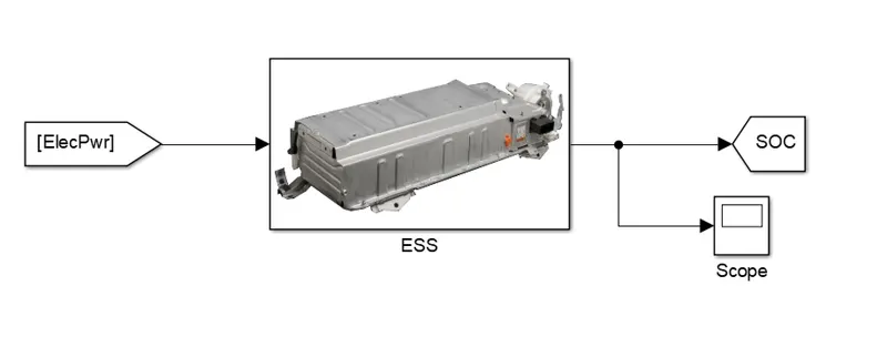
ESS Unit :

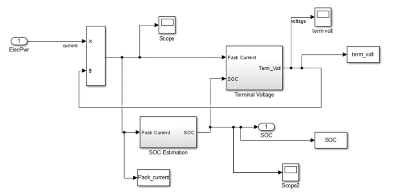
In this we give input as power then it multiply and give to pack current. Then from SOC estimation meet output SOC its give to terminal voltage as input and then meet terminal voltage as output.

Terminal Voltage :

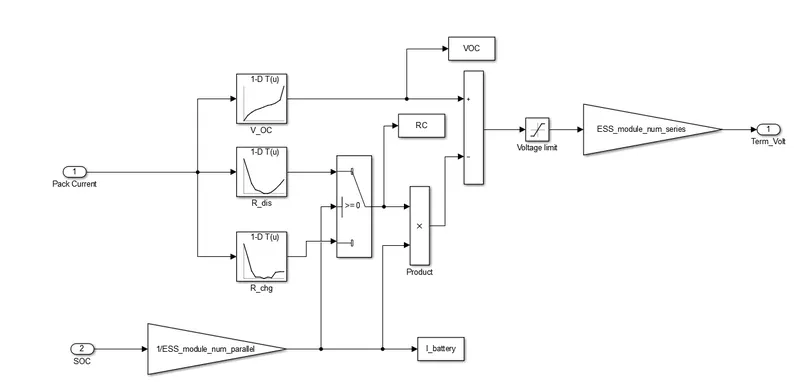
In this unit we use input SOC it is connected to 1D lookup table 1st table variable interpolated as state of charge and open voltage circuit. In 2nd lookup table is for the discharge resistance to the soc. And the 3rd lookup table is made of charging resistance to the soc states. Then it is passed through the switch block for controlling therushold then it give voltage limits as max volts to get terminal voltage.

SOC Estimation :

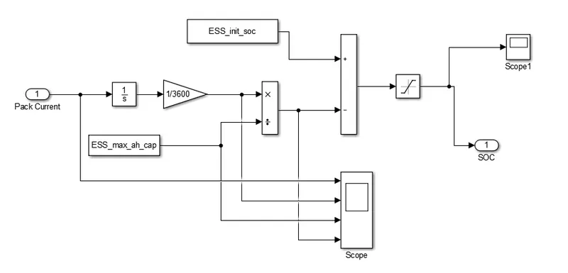
In this we integrate pack current and convert it rad to amp then saturated and meet SOC. and this current is divided by the maximum current capacity and it move to seperated by initial soc to get the final soc.

MATLAB Post Processing code :

The MATLAB script " Project2_ProcessingFile" is used to analyze the data from the simulink model and to generate plots. After the simulink vehicle model is run some of the data are sent to the workspace which is used to plot different parameters for the study of conventional vehicle in MATLAB.

%%%%%%%%%%%%%%%%%%%%%%%%%%%%%%%%%%%%%%%%%%%%%%%%%%%%%%%%%%%%%%%%%%%%%
%% Skill-Lync -> Hybrid Drives Development
% Project - Hybrid Vehicle Model
% By: Kaviyarasan K

% Description:
% The following file is to used with the Initialization file and Simulink
% results for post-processing of the data.

%% Post-Processing File
%  File for post-processing the Hybrid Vehicle simulation model data

close all;
%% Renaming variables
Time = tout;
Acc_Pdl = Acc_Pdl;              % Accelerator pedal [%]
Brk_Pdl = Brk_Pdl;              % Brake pedal [%]
Gear_Cmd = Gear_Cmd;            % Transmission gear
Trans_In_Spd = Trans_In_Spd*30/pi;  % Transmission input speed [rpm]
Trans_Out_Spd = Trans_Out_Spd*30/pi;% Transmission output speed [rpm]
Eng_Trq = Eng_Trq;              % Engine brake torque [Nm]
Eng_Spd = Eng_Spd*30/pi;        % Engine speed [rpm]
Eng_Fuel_Consump = Eng_Fuel_Consumption;    % Engine fuel consumption [g]
Enf_Fuel_Rate = Eng_Fuel_Rate;  % Engine Fuel COnsumption rate [g/s]
Veh_Dist = Veh_Dist/1000;       % Distance traveled by vehicle [km]
Veh_Spd = Veh_Spd*18/5;         % Vehicle speed [kmph]
WheelSpd = (Veh_Spd.*60)./(2.*pi.*Rw);  % Wheel rpm
Desired_Spd = Desired_Velocity  % Desired Speed [kmph]
EM_Speed = EMSpd                % Electical Motor Speed
EM_Power = EMPwr                % Electical Motor Power
EM_Torque = EMTrq               % Electical Motor Torque
Term_Volt = term_volt           % Terminal Voltage of Battery
Soc = SOC                       % State of charge
Pack_Current = Pack_current     % Pack Current of Battery

%% Data Analysis
Eng_Pwr = Eng_Spd.*pi./30.*Eng_Trq./1000;   % Engine brake power [kW]
rho_petrol = 0.7197;                        % Density of petrol [kg/L]
kmpl = Veh_Dist(end)/(Eng_Fuel_Consump(end)/1000/rho_petrol);    % Fuel economy [kmpl] 

%% Plotting vehicle characteristics time trace

% Plot: Transmission Input and Output, Wheel Speed
figure(1)
plot(Time, Trans_In_Spd, 'linewidth', 2, 'Color', 'green');
hold on;
plot(Time, Trans_Out_Spd, 'linewidth', 2, 'Color', 'black');
hold on;
plot(Time, WheelSpd, 'linewidth', 2, 'Color', 'red');
ylabel('Speed [rpm]');
xlabel('Time [s]');
xlim([0, Time(end)]);
legend('Transmission Input','Transmission Output','Wheel Speed');
grid on;

% Plot: Engine Torque, Engine Power, Fuel Rate & Fuel Consumption
figure (2)
subplot(4,1,1)
plot(Time, Eng_Trq, 'linewidth',2);
xlabel('Time [s]');
ylabel('Torque [Nm]');
legend('Engine Torque');
grid on;
xlim([0, Time(end)]);

subplot(4,1,2)
plot(Time, Eng_Pwr, 'linewidth',2);
xlabel('Time [s]');
ylabel('Power [Nm]');
legend('Engine Power');
grid on;
xlim([0, Time(end)]);

subplot(4,1,3)
plot(Time, Enf_Fuel_Rate, 'linewidth',2);
xlabel('Time [s]');
ylabel('Fuel Rate [%]');
legend('Engine Fuel Rate');
grid on;
xlim([0, Time(end)]);

subplot(4,1,4)
plot(Time, Eng_Fuel_Consump, 'linewidth',2);
xlabel('Time [s]');
ylabel('Fuel Consumption');
legend('Engine Fuel Consumption');
grid on;
xlim([0, Time(end)]);


% Plot: Accelerator & Brake Pedal, Gear, Vehicle actual & desired speed,
% Vehicle DIstance
figure (3)
subplot(5,1,1)
plot(Time, Acc_Pdl, 'linewidth',2);
hold on;
plot(Time, Brk_Pdl, 'linewidth',2);
xlabel('Time [s]');
ylabel('Pedal [%]');
xlim([0, Time(end)]);
legend('Accel','Brake');
title('Acceleration and Brake Pedal wrt Time')
grid on;

subplot(5,1,2)
hold on;
grid on;
plot(Time, Gear_Cmd, 'linewidth',2);
xlim([0, Time(end)]);
xlabel('Time [s]');
ylabel('Gear Change');
legend('Gear Change');
title('Gear Command wrt Time')

subplot(5,1,3)
hold on;
grid on;
plot(Time, Veh_Spd, 'linewidth',2);
legend('Actual Spd')
title('Actual Speed of Vehicle');
xlim([0, Time(end)]);
xlabel('Time [s]');
ylabel('Speed [kmph]');

subplot(5,1,4)
hold on;
grid on;
plot(Time, Desired_Spd, 'linewidth',2);
title('Desired Speed of Vehicle');
legend('Desired Spd')
xlim([0, Time(end)]);
xlabel('Time [s]');
ylabel('Speed [kmph]');

subplot(5,1,5)
hold on;
grid on;
plot(Time, Veh_Dist, 'linewidth',2);
title('Vehicle Distance')
legend('Distance');
xlim([0, Time(end)]);
xlabel('Time [s]');
ylabel('Distance [km]');


%% Plotting engine operating points on engine fuel map
figure('Name','Engine Operating Points');
hold on
grid on
title('Engine Operating Points','fontsize',12);
p1=plot(Eng_map_spd*30/pi,Eng_max_trq,'linewidth',2,'color','r');
p2=line([Eng_map_spd(end)*30/pi Eng_map_spd(end)*30/pi],[0 Eng_max_trq(end)]);
set(p2,'linewidth',1,'linestyle','--','color','k');
p3=line([Eng_map_spd(1)*30/pi Eng_map_spd(1)*30/pi],[0 Eng_max_trq(1)]);
set(p3,'linewidth',1,'linestyle','--','color','k');
[c,h] = contour(Eng_map_spd'*30/pi,Eng_map_trq,Eng_fuel_map');
clabel(c,h);
xlabel('Engine Speed [rpm]');
ylabel('Engine Torque [Nm]');
title('Engine Fuel Consumption Map [g/s]');
legend([p1 p4],{'Max Curve','Operating Points'});
axis([Eng_map_spd(1)*30/pi Eng_map_spd(end)*30/pi 0 Eng_map_trq(end)]);

%% plot motor speed, torque, motor input power using subplots.

figure(5)
subplot(3,1,1)
plot(Time, EM_power, 'linewidth',2);
xlim([0, Time(end)]);
xlabel('Time [s]');
ylabel('power [w]');
legend('Electric Motor Power');
grid on

subplot(3,1,2)
plot(Time, EM_torque, 'linewidth',2);
xlim([0, Time(end)]);
xlabel('Time [s]');
ylabel('Torque [Nm]');
legend('Electric Motor Torque');
grid on

subplot(3,1,3)
plot(Time, EM_speed, 'linewidth',2);
xlim([0, Time(end)]);
xlabel('Time [s]');
ylabel('Speed [rpm]');
legend('Electric Motor Speed');
grid on

%% Plot pack voltage, current and SOC using subplots.

figure(6)
subplot(3,1,1)
plot(Time, Pack_current, 'linewidth',2);
xlim([0, Time(end)]);
xlabel('Time [s]');
ylabel('Current [W]');
legend('Pack Current');
grid on

subplot(3,1,2)
plot(Time, State_of_charge, 'linewidth',2);
xlim([0, Time(end)]);
xlabel('Time [s]');
ylabel('Charge [%]');
legend('State of Charge');
grid on

subplot(3,1,3)
plot(Time, Term_Voltage, 'linewidth',2);
xlim([0, Time(end)]);
xlabel('Time [s]');
ylabel('Voltage [V]');
legend('Terminal Voltage');
grid on

%% Plot the motor operating points on the motor input power map, with the motor max torque curve
figure('Name','Electric Motor Operating Points');
hold on
grid on
title('Electric Motor Operating Points','fontsize',12);
p1=plot(EM_map_spd*30/pi,EM_max_trq,'linewidth',2,'color','r');
p4=plot(EM_map_spd*30/pi,EM_max_gen_trq,'linewidth',2,'color','b');
p2=line([EM_map_spd(end)*30/pi EM_map_spd(end)*30/pi],[0 Eng_max_trq(end)]);
set(p2,'linewidth',1,'linestyle','--','color','k');
p3=line([EM_map_spd(1)*30/pi EM_map_spd(1)*30/pi],[EM_map_gen_trq(1) Eng_max_trq(1)]);
set(p3,'linewidth',1,'linestyle','--','color','k');
[c,h] = contour(EM_map_spd'*30/pi,EM_map_trq,EM_inpwr_map');
clabel(c,h);
xlabel('Motor Speed [rpm]');
ylabel('Motor Torque [Nm]');
title('Motor Input Power Map');
legend([p1 p4],{'Max Curve','Regen Curve','Operating Points'});
axis([EM_map_spd(1)*30/pi EM_map_spd(end)*30/pi EM_map_gen_trq(1) EM_map_trq(1)]);

For the study of the developed vehicle model with various drive cycle, the code to plot the following relations are made,

• The time trace for engine, transmission input and output speed on one plot.
• The engine torque, engine power, fuel rate and fuel consumption using subplots.
• The accelerator and brake pedal, gear command, vehicle desired and acutual speed, vehicle distance using subplots.
• The engine operating points on the engine fuel map.
• The motor speed, torque, motor input power using subplot.
• The pack voltage, current and SOC using subplot.
• The motor operating ponits on the motor input power map.

Study of the developed model for UDDS and HWEET drive cycle :

Fuel Economical Numbers :

Project 2 :

The Fuel Economical Number for UDDS cycle is 15.077

The Fuel Economical Number for HWFET cycle is 17.161

Project 1 :

The Fuel Economical Number for UDDS cycle is 14.205

The Fuel Economical Number for HWFET cycle is 16.501

As we see the fuel economy number is high in HWFET when compared to UDDS cycle. Because in urbon driving the vehicle encounters more traffic and it has to stop for small distance and it conumes more fuel.

As we see the fuel economy number for project 2 is little bit higer than the project 1. Because of implementing the electric motor as it is P1 hybrid vehicle. It may not much variation in the fuel economy but as we improve other architecture it will increase by huge amount.

Plots for various speed [rpm] :

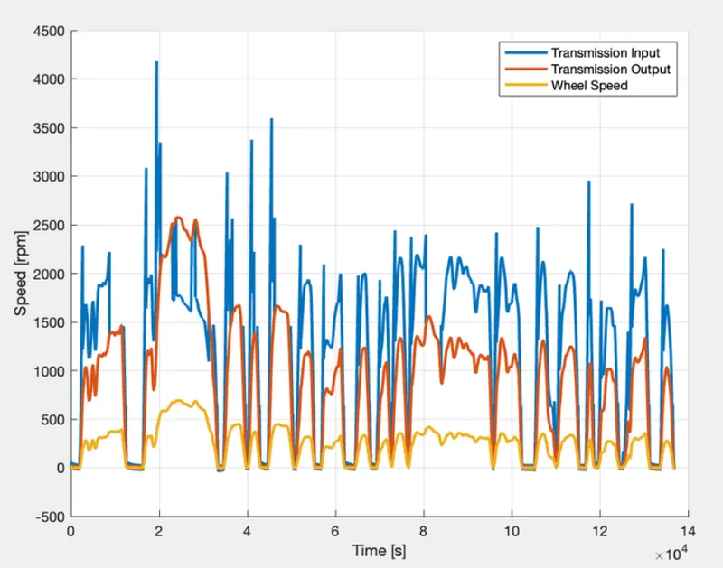
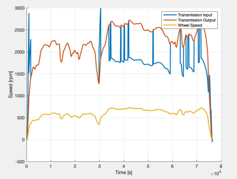
This first plot is for time trace for engine speed, transmission input speed, transmission output speed. From this plot we see the transmission input speed is always high and wheel speed(Yellow curve) is low when compaired to input speed (blue curve) this is happen from the units persent between this two. The transmission loss and the differential loss are the reason for this variation.

For UDDS drive cycle,

For HWFET drive cycle,

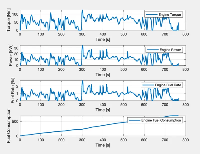
Plots for engine torque, power, fuel rate and fuel consumption :

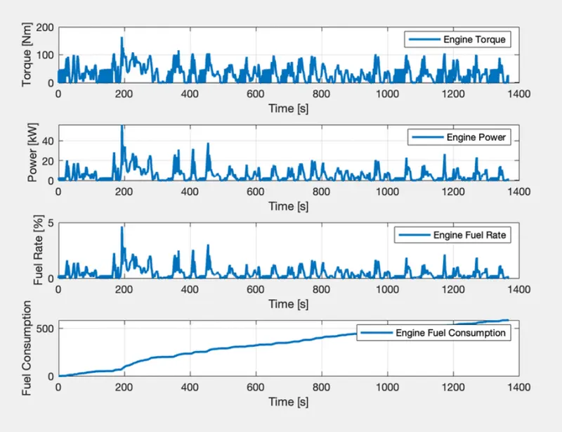
The drive cycle velocity for HWFET is more in the higer range than the UDDS. The power requirement is directly proportional to the power of three for the aerodynamic drag and directly proportional to the rolling and grading resistance. Since, the proportion of higher velocity is more predominant in HWFET the vehicle requires more power to run HWFET than UDDS which means that, the fuel consumption of UDDS is less than HWFET even through the drive cycle time is more for UDDS.

For UDDS drive cycle,

For HWFET drive cycle,

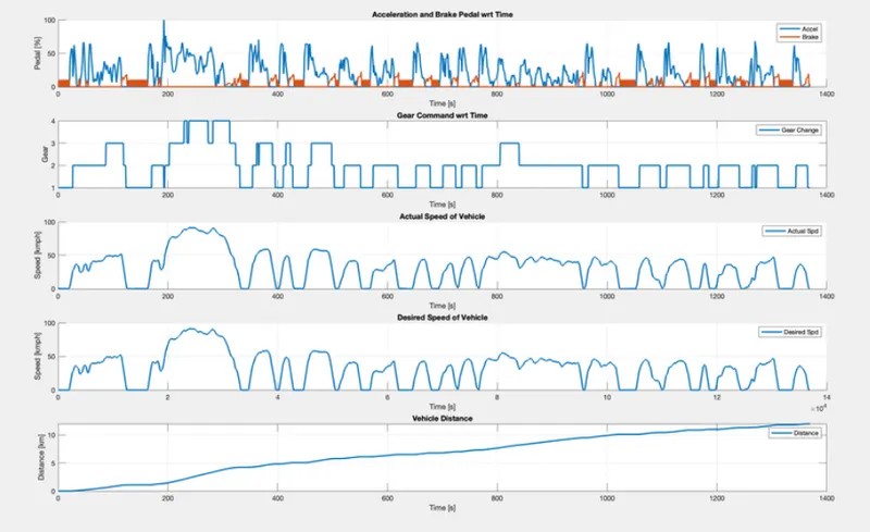
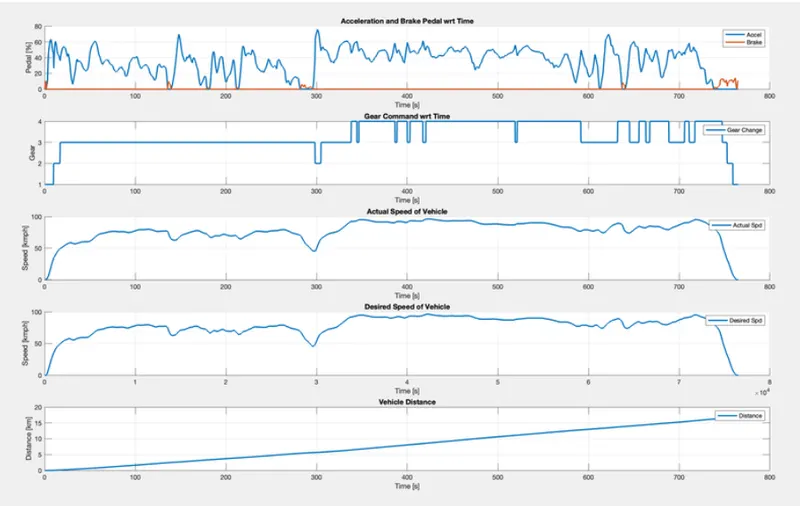
Plots for Acceleration, Brake pedal, Gear position and distance :

The UDDS drive cycle seems to have more prominent varying velocity over time than HWFET. Therefore, more brake pedal has to be used for UDDS than HWFET which can be observed from the first subplot. The more the brake padal is pressed. the more will be the energy loss, which in turn means that less will be the fuel economy number.

The second plot is shows the current gear position of the vehicle as the required speed it change the gear automatically by the automatic transmission system present in this system. Third plot is shows that the current velocity of the vehicle.

For UDDS drive cycle,

For HWFET drive cycle,

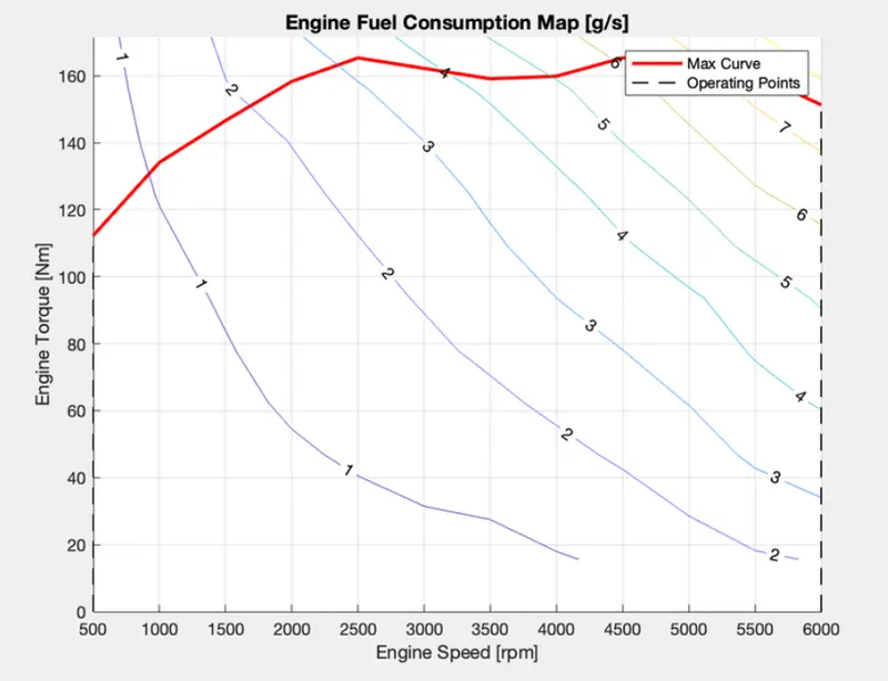
Plots for Engine fuel consumption map :

For UDDS drive cycle,

For HWFET drive cycle,

Plots for motor Speed, Torque and Power :

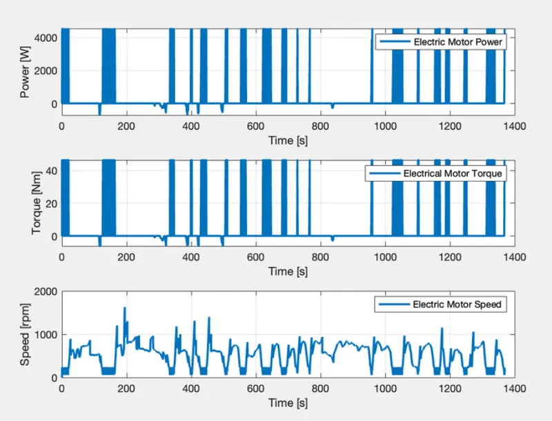
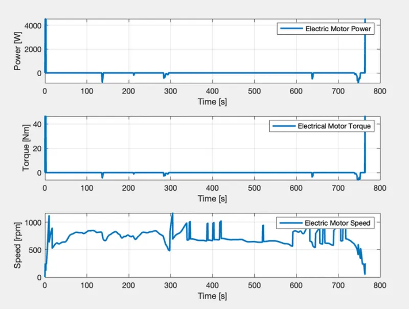
This plots for the motor speed and the torque. this electic motor used in low speed drive conditions as we mentioned in the mode logic unit. so at the urbon drive has lot of low speed drive so it used lot of motor power in UDDS cycle when compare to HWFET cycle as shown in the plots.

For UDDS drive cycle,

For HWFET drive cycle,

Plots for Pack voltage, Current and SOC of Battery :

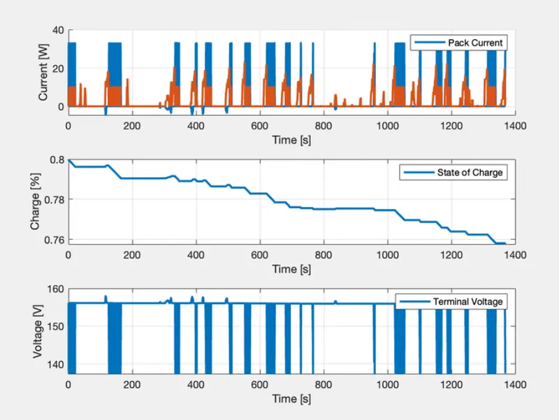
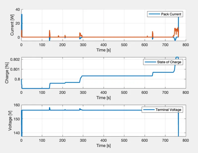
This plot is for the pack current and the SOC. The red curves are the regen braking due to this the brake energy is converted into electrical energy and store in the battery. The second subplot is shows the state of charge with the time trace.

For UDDS drive cycle,

For HWFET drive cycle,

Plots for Motor Input Power Map :

For UDDS drive cycle,

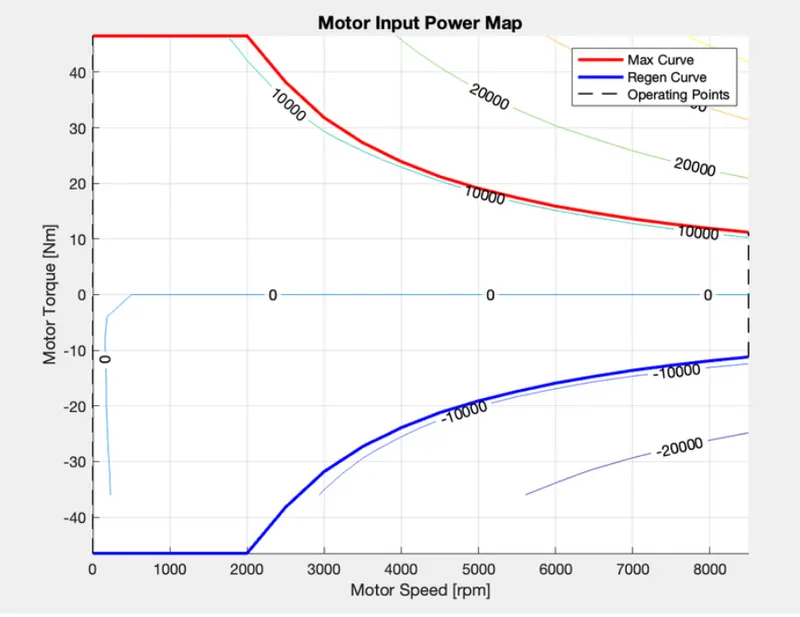
For HWFET drive cycle,

Conclusion :

The MATLAB script for both initializing and post processing has be successfully made, and a forward energy based fuel consumption simulink model of a P1 type Hybrid electric Vehicle is also developed successfully and the functions are checked. The comparative study of using USSD and HWFET drive cycles for the developed vehicle model is analyzed.