Project: Forward Energy-Based Model of a P1 Hybrid Vehicle [MATLAB & SIMULINK]

Aim:

To develop a forward energy-based fuel consumption model of a P1 hybrid vehicle in MATLAB and Simulink.

Theory:

Energy Based Models - Model Structure
There are two basic types of structure for the energy-based models:

1. Forward Model: Dynamic simulation of the system
2. Backward Model: Quasi-Static simulation of the system.

Forward models simulate from source to sink, that is, from the input to the engine to the wheels, in order to assess vehicle performance.
Backward models simulate from the source to the sink, i.e. the input is the vehicle speed and acceleration, and the engine input is calculated backwards.

Forward Models
Forward models are utilized for detailed simulations, whereas dynamic models are used for forward models (refer Figure 1). The input is force/torque/power, and the outputs are the vehicle state variables velocity and acceleration. Because physical casualty makes models and simulations more realistic, they are better for control development. To achieve the desired vehicle state, there is a feedback loop. Because of the dynamics, the simulation is slower, and the approach is mostly used to model a vehicle drive cycle and study the system's dynamic behavior. Significantly aids in the management of development.

Figure 1: Forward Model

Backward Models
Backward models are calculated in a quasi-static manner. The inputs include vehicle conditions like velocity and acceleration, whereas the output is the force, torque, and power required at the source, i.e. the engine. They are simple and quick to use, making them ideal for quick computations and comparisons. They lack dynamics, and the method is mostly used to calculate simple fuel consumption and optimize energy management (refer Figure 2).

Figure 2: Backward Model

Conventional Vehicle
Conventional vehicles use an internal combustion engine fueled by gasoline or diesel, to power the wheels. The heat engine works on the premise of releasing heat by combusting fuel with an oxidizer in a combustion chamber to produce expanding gases that push against a piston, producing force and torque. The chemical energy of fuel is transformed into heat energy in internal combustion (IC) engines to produce meaningful mechanical work. Four stroke reciprocating engines are the most prevalent type of engine. Internal combustion engines and conventional vehicles use ideal thermodynamic cycles like the Otto Cycle, Diesel Cycle, Over expanded cycle, and so on.

P1 Hybrid Architecture (Crankshaft mounted electric machine)
The P1 architecture, with the electric machine connected directly to the crankshaft, is the solution adopted by Honda on their first generation Integrated Motor Assist (IMA) technology. During vehicle slowdown, the electric motor acts as a generator, as an engine starter, and as a motor (to help the engine) during vehicle accelerations.

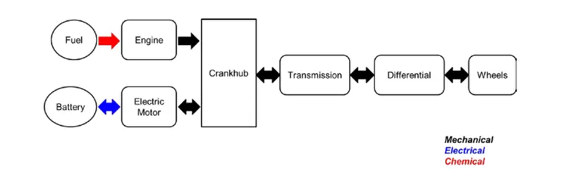
Figure 3: Block Diagram Representation of P1 Hybrid Architecture.

One of the most significant advantages of this system is that the electric motor may deliver higher torque than the BiSG due to the absence of a belt (due to slip). The torque requirements on the electric motor can be rather demanding because there is no speed / torque ratio between the electric machine and the crankshaft.

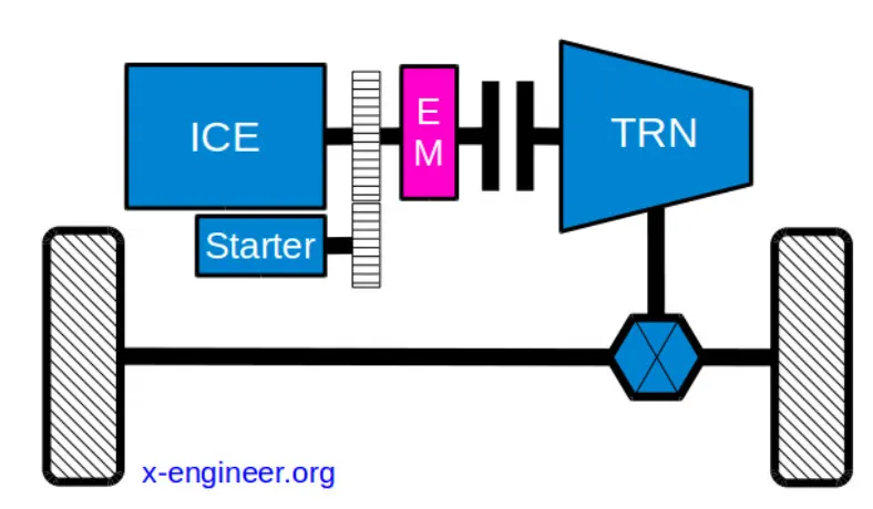
Figure 4: P1 Architecture - Integrated Starter Generator [x-engineer]

The removal of the belt drive is the key benefit of a P1 mild hybrid architecture over a P0. This means that efficiency improves slightly (no more belt losses), and electric machine torque amplitude and response can be increased (no more belt slip).

Although the functions (modes) performed by this mild hybrid topology are comparable to those of a BiSG (P0), P1 configurations have two major drawbacks: more cost and greater influence on existing vehicle architecture. As a result, vehicle manufacturers and system suppliers are not investing in the development of a crankshaft-mounted integrated starter generator solution for MHEVs.

The two main examples of P1 MHEV architectures are:

• Honda Insight Hybrid 2009 (with Integrated Motor Assist technology)
• Mercedes Benz S400 Bluehybrid 2010

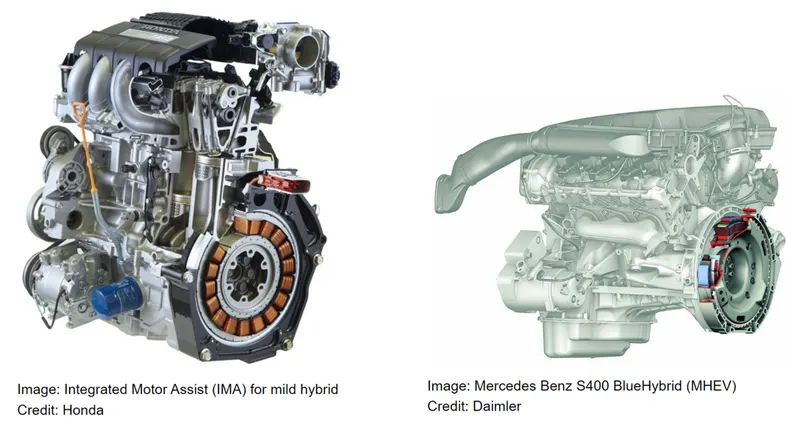
Figure 5: Examples of P1 MHEV Architecture [x-engineer]

Both P0 and P1 mild hybrid configurations have the electric machines on the engine side, without the possibility of mechanical disconnection. This makes torque boosting and energy recuperation not very efficient because of the torque losses. Moreover, recuperating electrical energy with the engine off, during coasting, is not possible.

The P2, P3 and P4 mild hybrid architectures are better in terms of energy flow efficiency, mainly because of the positioning of the electric machine. In these types of configurations, the electric machine is positioned after the driveline connecting device (clutch), on the input shaft of the transmission (P2), on the output shaft of the transmission (P3) or on the rear differential (P4).

Energy Demand for Drive Cycle
Energy demand at the wheel, due to a drive cycle can be computed. The force at the wheels are given by,
`F_"tractive"=M(dV)/dt+1/2ρ_aA_fC_d(V±V_w)^2+C_rMgcos(α)+Mgsin(α)`
where, `M` is the vehicle mass [`kg`], `V` is the vehicle velocity [`m//s`], `rho_a` is the air density [`kg//m^3`], `A_f` is the frontal area of the vehicle [`m^2`], `C_d` is the drag coefficient, `V_w` is the wind velocity [`m//s`], `C_r` is the rolling coefficient, `g` is the acceleration due to gravity [`m//s^2`], and `alpha` is the road inclination.

The power at the wheels is given by,
`P_"tractive"=F_"tractive"⋅V`
`P_"tractive"=MV(dV)/dt+1/2ρ_aA_fC_dV(V±Vw)^2+C_rVMgcos(α)+VMgsin(α)`

Assuming no grade (`alpha`= 0) and no headwind (`V_w`= 0),
`P_"tractive"=P_w=MV(dV)/dt+1/2ρ_aA_fC_dV^3+C_rMgV`

Energy demand for the drive cycle is computed by integrating power over time for the entire cycle,
`E_w=∫P_wdt=∫MV(dV)/dtdt+∫1/2ρ_aA_fC_dV^3dt+∫C_rMgVdt`

Assuming mass, air density, drag coefficient, frontal area, rolling resistance coefficient and acceleration due to gravity are constant for the drive cycle,
`E_w=M∫V(dV)/dtdt+1/2ρ_aA_fC_d∫V^3dt+C_rMg∫Vdt`
`E_w=k_i∫V(dV)/dtdt+k_a∫V^3dt+k_r∫Vdt`
where, `k_i` is the coefficient of inertial resistance, `k_a` is the coefficient of aerodynamic drag, and `k_r` is the coefficient of rolling resistance, and they are given by,
`k_i=M`
`k_a=1/2ρ_aA_fC_d`
`k_r=C_rMg`

The energy component `[k_i∫V(dV)/dtdt]` is the kinetic energy of the vehicle and is always 0 over the entire drive cycle. For a conservative system (i.e. no dissipative forces), the aerodynamic drag and rolling resistance component of the energy will also be 0. Also, when `P_w<0`, the energy is absorbed by the brakes. This can potentially be recaptured through regenerative braking.

To calculate energy, the integrals can be discretized. Generally, time step of 1 sec is sufficient for the drive cycles.
`E_w=k_i∑_iV(i)(dV(i))/dtΔt+k_a∑_iV^3(i)Δt+k_r∑_iV(i)Δt`

Powertrain Sizing
Based on the individual power requirement for the drive cycle, effect of aerodynamic drag, rolling resistance and inertial component can be analyzed. High power is required to sustain high vehicle speeds, due to the increasing drag component. From the overall power plot, the maximum positive power is the power that needs to be provided at the wheels by the powertrain to complete the cycle. This sets the minimum powertrain sizing requirement. Additionally, if all the potential braking energy is to be captured, then the regenerative unit must be at least be designed to handle maximum negative power for the cycle.

Drive Cycle Development
Although the regulatory drive cycles are important as they form part of the certification processes and are well developed, they only form a part of the vehicle development process as they do not represent all the driving conditions that the manufacturer wants to develop for. The manufacturer might have tests representing different driving scenarios and also might have more aggressive tests depending on the application. Therefore, for an optimized design and to minimize the development time, it is important to be able to develop drive cycles, which can be either used in simulations or vehicle testing. Cycles that depend on certain vehicle capability can be relatively developed. For example, to test the vehicle towing capacity upto a grade, need to specify towing load, speed, grade and time of operation. Multiple cycles can be added to test the capability of the powertrain. For developing a drive cycle from a real world driving trip, the data is divided into kinematic sequences. The sequences are classified into distinct clusters. Probability of the occurrence of each type of sequence during a certain type of driving trip is calculated. Drive cycles are constructed by randomly selecting sequence based on their probabilities and a cycle is built based on the selection of cycle type, minimum cycle duration, distance, number of stops, average and top speeds, etc.

Energy Based Models - Element Models
To model the internal physical properties of the element and the losses, there are two kinds of approaches: Map based models and Analytical models.

1. Map based models:
   Elements are modeled using maps, which characterize the relationship between the input & output and output & losses etc.
2. Analytical models:
   Elements are modeled using the physical equations, that represent the internal dynamics.

Objectives:

1. Understand the concept of forward energy-based fuel consumption model of a P1 Hybrid Architecture.
2. Understand the functioning various vehicle components including engine, electric motor, crank hub, torque converter, transmission system, longitudinal dynamics, etc.
3. Development of a Matlab script used to load all the variables required for running the Simulink model.
4. Development of the Simulink model of the vehicle.
5. Development of a MATLAB script to do post-process calculations and generate results and plots.
6. Analyzing the results.

MATLAB Initializing Code:

A MATLAB script “Project2_InitFile.m” is to load the variable to the workspace that is to be used for the further calculation/processing for the Simulink model. A typical midsize car with a 1.9L engine and a 4-speed automatic transmission is considered. Honda Insight motor and battery are considered for this project for the hybrid part. Data is taken from ADVISOR data base developed by NREL, USA. Transmission shift map and controller is taken from Matlab/Simulink example database.

Motor:	10 kW PMSM
Battery:	6Ah 154V NiMH battery pack

%%%%%%%%%%%%%%%%%%%%%%%%%%%%%%%%%%%%%%%%%%%%%%%%%%%%%%%%%%%%%%%%%%%%%
%% Skill-Lync -> Hybrid Drives Development
% Project - P1 hybrid vehicle Model
% By: Jibin Jafar

%% Description:
% Initialization File
% Initialization file for loading the variables for the Conventional vehicle simulation model


clear all;
close all;
clc;

%% Vehicle Parameters
M = 1500;       % Vehicle weight [kg]
Cr = 0.015;     % Rolling resistance coefficient
Rw = 0.35;      % Rolling radius [m]
Cd = 0.33;      % Drag coefficient
Af = 2;         % Frontal area [m2]
rhoa = 1.225;   % Air density [kg/m3]
Vwind = 0;      % Wind velocity [kmph]
g = 9.81;       % Gravitational acceleration [m/s2]
theta = 0;      % Slope [deg]
myu_road_tire = 1; % Coefficient of friction between tire - road interface

%% Powertrain Parameters 
FDR = 3.73;                         % Final Drive Ratio / Diff Ratio
DiffEff = 0.99;                     % Differential efficiency (assumed independent of operating conditions)

NumGear = 4;                        % Number of gears in transmission
TransGear = [1:NumGear];            % Transmission Gears
TransRatio = [3.06, 1.62, 1, 0.7];  % Corresponding Transmission ratios
TransEff = 0.90;                    % Transmission efficiency (assumed independent of operating conditions)

TC_SR = [0, .5, .6, .7, .8, .87, .92, .94, .96, .97, 1];   % Torque Converter Speed Ratio (Matlab default) -> TurbSpd/PumpSpd  
TC_TR = [2.232, 1.5462, 1.4058, 1.2746, 1.1528, 1.0732, 1.0192, 1, 1, 1, 1];   % Torque Converter Torque Ratio (Matlab default) -> TurbTrq/PumpTrq
TC_Cf = 1e-4 * [.72558, .66322, .63463, .59042, .51331, .4144, .29287, .22444, .12186, .04386, 0]; % Torque Converter Capacity Factor (Matlab default) -> PumpTrq/PumpSpd^2 [Nm/rpm^2]

load Vehicle_Data/Engine_data_1_9L_Saturn_95kW
load Vehicle_Data/Trans_Shift_map
load Vehicle_Data/EM_Honda_Insight_10kW
load Vehicle_Data/ESS_NiMH6


ESS_init_soc = 0.8;
ESS_soc_max = 0.9;
ESS_soc_min = 0.6;


%% Driver Parameters
Kp = 10;                    % P gain for driver PI model
Ki = 1;                     % I gain for driver PI model
Drive_Cycle_Select = 2;     % Drive cycle selection

% Drive cycle values in m/s

%% Inputting the desired DriveCycle
Drive_Cycle_Select = input(sprintf('Select a Drive Cycle: n 1. UDDS n 2. HWFET n 3. FTP n 4. US06 n 5. NEDC n 6. WLTP n Your selection is: '));
% Drive cycle values in m/s

% Loading Drive Cycle values. Variables: cyc_time, cyc_vel
if Drive_Cycle_Select == 1
    load DriveCycles/UDDS;
    
elseif Drive_Cycle_Select == 2
    load DriveCycles/HWFET;
    
elseif Drive_Cycle_Select == 3
    load DriveCycles/FTP;
    
elseif Drive_Cycle_Select == 4
    load DriveCycles/US06;
    
elseif Drive_Cycle_Select == 5
    load DriveCycles/NEDC;
    
elseif Drive_Cycle_Select == 6
    load DriveCycles/WLTP;
 
end

time_end = cyc_time(end);   %End time from drive cycle
vel_end = cyc_vel(end);     %End Velocity from drive cycle

%% Running Simulink Model 
sim('Project2_P1VehicleModel');   % Run Simulink model

%% Running Post Processing Script
Project2_ProcessingFile;        % Run Post processing Matlab script

Each step of the code is explained with comments.

The code assigns various vehicle, powertrain and driver parameters. The MATLAB file "Engine_data_1_9L_Saturn_95kW" loads the engine parameters including Engine efficiency map, Engine fuel map, Engine Inertia, Engine map speed, Engine map torque and Engine torque and maximum torque values. The MATLAB file "Trans_Shift_map" provides the necessary data required for the control logic of Transmission control unit. The file "EM_Honda_Insight_10kW" provides the electric motor parameters including its efficiency map, inertia value, input power map, motor map speed, motor map torque, maximum torque and regenerative torque values. The file "ESS_NiMH6" provides all necessary data of the battery including max and min volts, max capacitance, SOC and initial voltage, etc. This code is designed such a way that it asks for the drive cycle that need to be used for the study and the user input decides the desired drive cycle for the study. The screenshot of the command window asking for the drive cycle of study is shown in Figure 6. For the chosen drive cycle, the Simulink vehicle model will be run automatically, and after that, MATLAB post processing script will be run automatically for providing the necessary plots for the study.

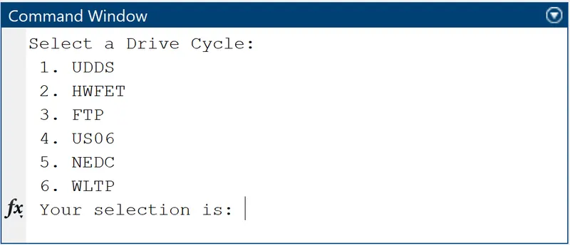
Figure 6: User interface for selecting drive cycle.

Simulink Vehicle Model:

The Simulink model consist of three main subsystems: Driver, Controller and Powertrain, as shown in Figure. The Driver subsytem generates the accelerator and brake pedal outputs to match the desired and actual vehicle speed. The Controller block represents the electronic control units, which generates the desired engine torque, desired transmission gear, desired electric motor torque, clutch lock-up signal and desired brake torque based on the driver inputs. The Powertrain subsytem represents the actual vehicle consisting of all vehicle components which inputs the control signals from Controller and provides actual vehicle motion characteristics.

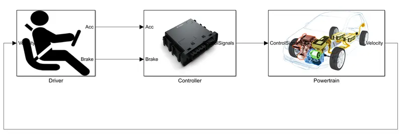
In brief, the Simulink model is modeled using a ‘Driver’ block, which is a basic PI controller that generates accelerator and brake pedal outputs to match the desired and actual vehicle speeds. The ‘Controller’ block is the brains of the vehicle, representing the electronic controls units. Based on the driver inputs, it generates desired engine and motor torque, desired transmission gear and desired brake torque. These inputs are fed to the ‘Powertrain’ block which represents the drivetrain of the vehicle. It consists of an ‘Engine’ and 'Electric Motor' connected to the ‘Automatic Transmission’ through a ‘Torque Converter’. The 'Electric Motor' is connected to 'Battery Model / ESS' where the battery parameters are found. The output of the transmission is connected to the ’Differential’, which powers the ‘Wheels’, that provides the tractive force for vehicle acceleration. The longitudinal dynamics of the vehicle along with the road load is represented in the ‘Vehicle Dynamics’ block. The solver selected is ode3 with a fixed step size of 0.01 sec.

• Driver Block
  
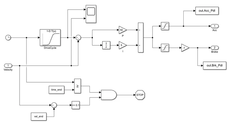
  This block is basically a PI controller. A PI Controller is a feedback control loop that calculates an error signal by taking the difference between the output of a system. It multiplies the error with constant gain for P and for I, it integrates and then multiply with a smaller gain. The constant value for P and I are found by trial-and-error method. Here, the error is the difference between the desired vehicle speed (from drive cycle) and the actual vehicle speed. The error could be positive or negative. The integrator block used keeps on adding the error is then divided into two since the driver block need to produce the signal for acceleration and brake pedal. The saturation block extracts the positive and negative signal as the acceleration pedal is passed on between the values 0 and 100, while for the brake pedal, the values between -100 and 0 are extracted, which means it provides the value between 0 and 100 percentage. This negative signal for the brake pedal is multiplied by -1 to make it a positive value. The scope is provided to compare the actual and desired speed. The sample scope output for the UDDS drive cycle is provided in Figure 7. For stopping the simulation when a set of conditions are satisfied, another set of blocks are provided. The comparative block compares the actual time and end time of drive cycle, similarly the current velocity is compared with the end velocity. If both conditions are satisfied, then the simulation is forcefully stopped. This is done in order to stop the simulation when drive cycle end independent of the drive cycle chosen as different drive cycle have different end time.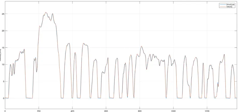
  
  
  Figure 7: Scope output for comparing velocities.
  
  
  
  
• Controller Block
  
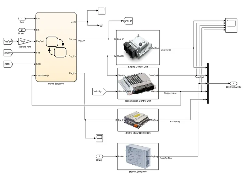
  The output of the driver block which is the acceleration and brake pedal signal is passed on to the Controller block. The controller block consists of three control units: Engine Control Unit, Transmission Control Unit, Electric Motor Control Unit and Brake Control Unit. All these data from the four Control Unit goes to the bus creator. The bus creator is used to combine all these five signals to a one signal. This combined signal is then sent to the Powertrain block. 'Model selection' logic controller is the supervisory controller . It is mainly used to graphically represent the main function of different states. It provides the input signals to the 'Engine Control Unit', 'Transmission Control Unit', 'Electric Motor Control Unit' and 'Brake Control Unit'. The Engine Control Unit accepts the Engine throttle signal from the driver block and converts it into the engine torque requirement signal which is to be passed to the powertrain block. Similarly, the Electric Motor Control unit and Brake Control Unit also convert the motor throttle signal and brake signal into respective motor torque requirement and brake torque requirement signals.
  
  
  
  • Mode Selection
    
    
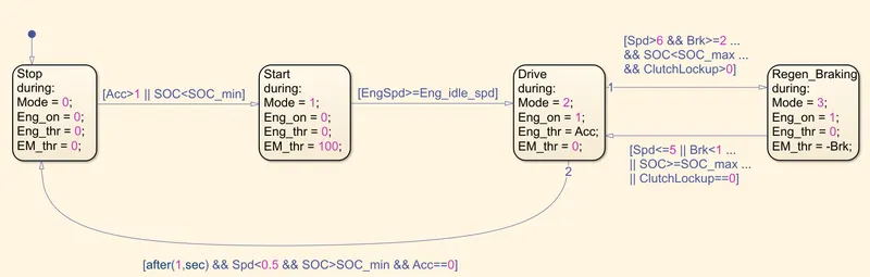
    The four different states are Stop, Start, Drive and Regen_Braking. Stop mode represents the engine is off. When acceleration is pressed or if the battery charge is less than intended, it moves to the state Start when the engine is on, but it does not necessarily mean that the engine provides the energy for motion. It moves to the Drive state if the engine speed is greater than idle speed and the engine status shows it is in ON condition and no power from the motor is used. When the vehicle moving at reasonable high speed and braking input is greater than 2, Regen_Braking status is enables where motor receives power. This happens only if battery charge is less than maximum capacity. Similarly, it is moved back to Drive state if any on this condition is not satisfied. During Drive state, if very low speed is detected and have enough battery capacity with no acceleration of vehicle, the state is directly changed to Stop.
    
    
    
  • Engine Control Unit
    
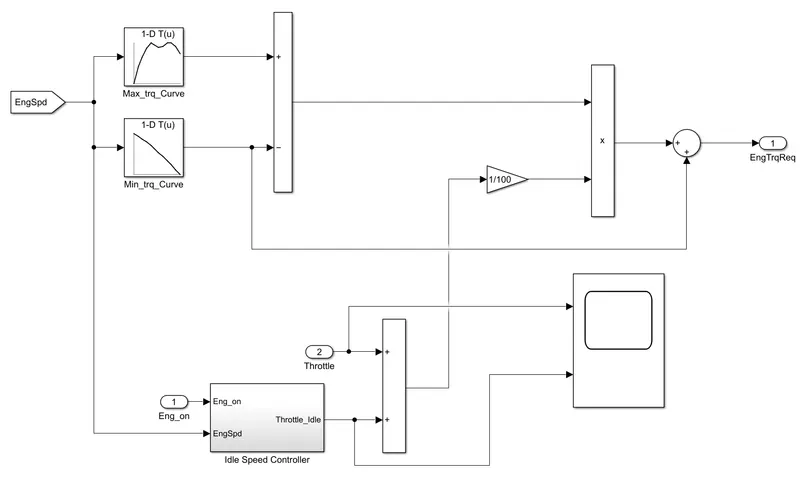
    The engine control unit has Idle Speed Controller to make sure that the engine is idling and doesn't go beyond idle speed. The signal from the Idle Speed controller is added to the throttle request from the Driver block is then converted into engine torque request based on the maximum and minimum torque curves made from 1D lookup table. A sample output from the scope for the UDDS drive cycle is shown in Figure 8.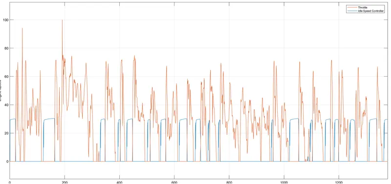
    
    
    
    Figure 8: Scope output for showing functionality of Idle Speed Controller.
    
    
    
    • Idle Speed Controller
      
      
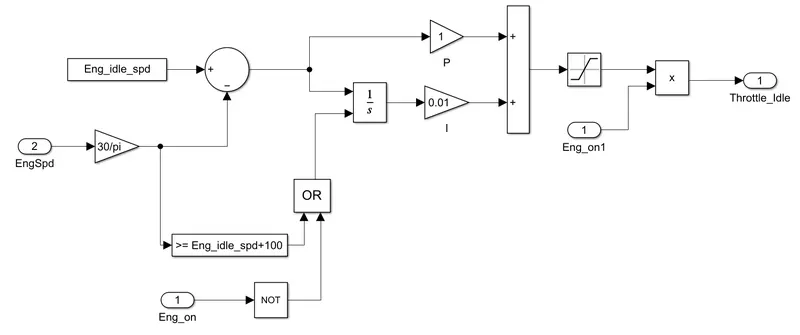
      The Idle Speed Controller is a PI Controller where the engine speed and the idle speed of the engine is compared. The error is then multiplied with constant P and the integrated error is multiplied with constant I. It gives out the required torque command to the engine block. The throttle input is combined with the idle speed throttle and gains with the torque output from the lookup table to estimate the torque input requirement for the engine. A condition is set using NOT conditional gate to ensure that it shows output only if the engine is ON. That is, Eng_on signal is implemented to eliminate the idle losses for the engine by eliminating the idle throttle for the engine off conditions.
      
      
      
  • Transmission Control Unit
    
    
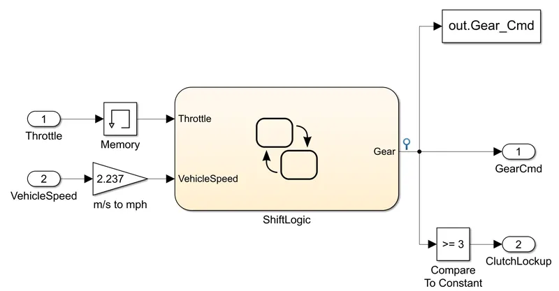
    It uses a state logic and provided the current gear of the vehicle. The state is defined by comparing the throttle signal and vehicle speed and it controls the gear shifting using the flow variable chart. The ShiftLogic is the logic control block for defining the gear.
    
    
    
    • ShiftLogic
      
      
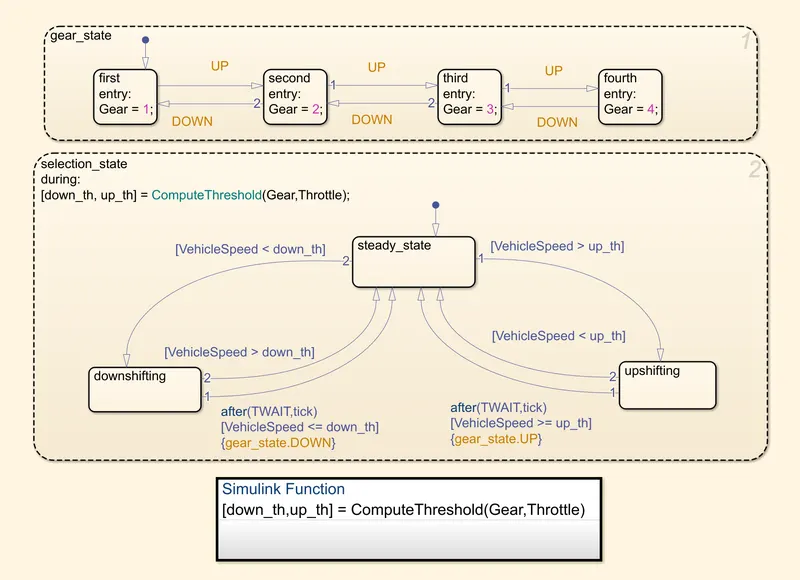
      The gear_state is defined between 4 states as the vehicle has four gears in total. The UP and DOWN values are calculated using another state selection_state. When in selection_gear state, a function ComputeThreshold is calculated where the inputs are Gear and Throttle. The output will be down_th and up_th for the function which are speed limits. The outputs from the function is fed in, then the downshift and upshift is done based on vehicle speed and the parameter inputs from matlab file Trans_Shift_map.
      
      
      
      • ComputeThreshold function
        
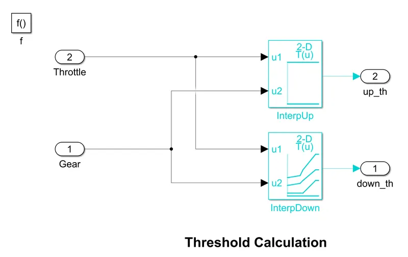
        The function uses lookup tables to find the transmission shifts and provides two outputs which feeds the selection_state.
        
        
        
  • Electric Motor Control Unit
    
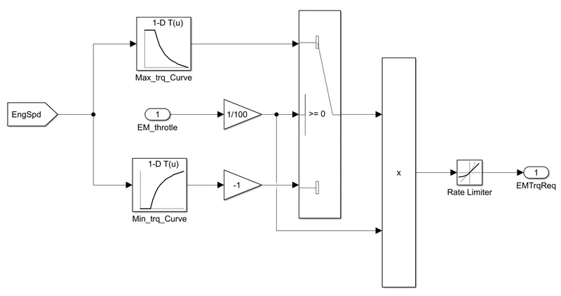
    The block provides the motor torque requirement by analyzing the engine torque and the motor max and min torque curves.
    
    
    
  • Brake Control Unit
    
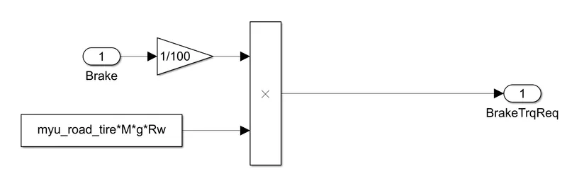
    The Brake pedal signal from the Driver block is multiplied with the maximum friction, which gives the maximum braking torque. The gain block is used convert to actual value from the percentage.
    
    
    
• Powertrain Block
  
  
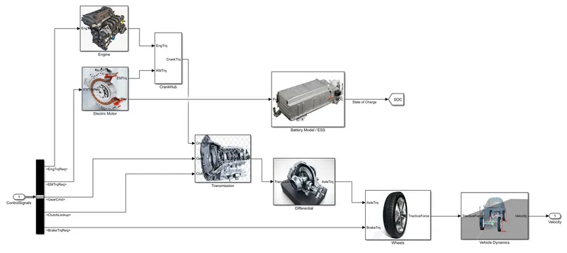
  The Powertrain block consists of eight main subsystems: Engine, Electric Motor, CrankHub, Battery Model / ESS, Transmission, Differential, Wheels and Vehicle Dynamics. The signals from the Controller block are extracted using the bus selector, which consists of the signal for Engine and Motor torque requirement, Gear command, and Brake Torque Requirement.
  
  
  
  • Engine
    
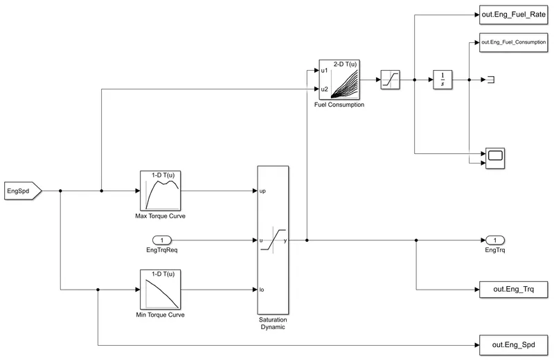
    The Engine blocks takes in Engine Torque requirement as input and it is compared with the maximum and minimum torque curve and is maintained between the required range using the saturation dynamic block. The maximum and minimum torque curve are found using the lookup table according to the engine speed from the data from the matlab file "Engine_data_1_9L_Saturn_95kW". The engine torque requirement after filtration is passed to the 2D lookup table along with engine speed where the fuel consumption rate is found. The saturation block ensures that the fuel rate value is positive and integrating it gives the total engine fuel consumption. The required parameters are transferred to the workspace using To Workspace blocks.
    
    
    
  • Electric Motor
    
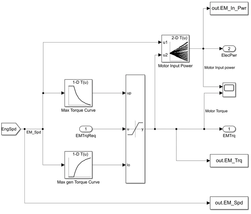
    Based on the engine speed, the required motor torque from the controller is saturated between maximum and minimum torque curves of the motor. The input electrical power of the motor is calculated using the 2D lookup table based on motor speed and torque. The motor characteristics are obtained from the MATLAB file "EM_Honda_Insight_10kW". A sample output from the scope for UDDS drive cycle is shown in Figure 9.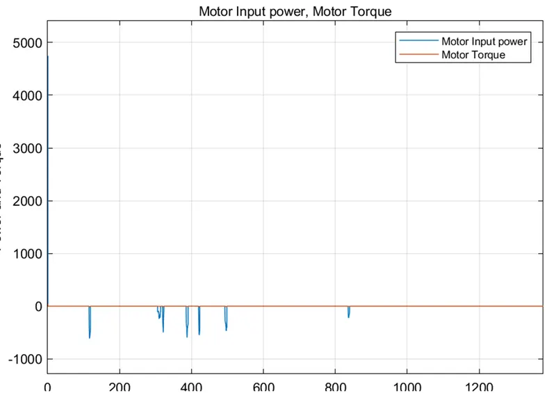
    
    
    
    Figure 9: Sample scope output for analysing the functionality of the motor
    
    
    
  • Crank Hub
    
    
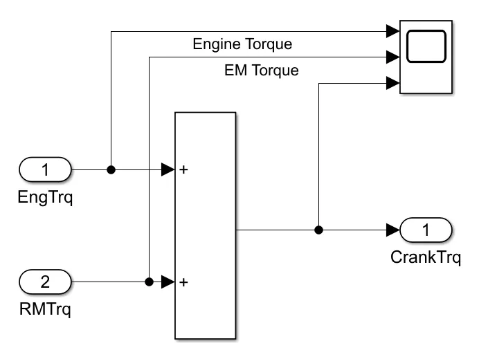
    This block adds up the Engine and the motor torque and is been passed to the transmission block as its input.
    
    
    
  • Battery Model / ESS
    
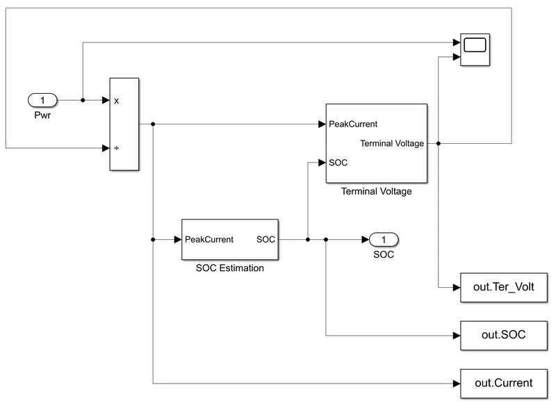
    This model has motor power requirement as the input. This is passed on to the SoC Estimation model, where the SoC of the battery model is calculated for each time. This calculated SoC and current data is passed on to the Terminal Voltage subsytem, where the terminal voltage is found. Further explanation of each subsystem is provided below. The found value of terminal voltage, SoC,and pack current are passed on to the Matlab model using the To Workspace block.
    
    
    
    • SOC Estimation
      
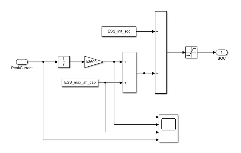
      `SOC(t)=SOC_0−int_0^t(I(t)dt)/(C_"nom")`
      The above equation is used for the calculation of SOC, where `SOC_0`is the SOC at initial condition at t=0, `I(t)` is the current that is drawn in the battery, and `C_"nom"` is the nominal capacity. The input data current is integrated and divided with 3600 in order to convert it in terms of joule, which is divided with `C_"nom"` which is provided in loaded ESS_NiMH6.mat file. The `SOC_0` is assumed to 80%, and the `SOC(t)` is calculated. The saturation block is used to ensure that the found SoC is within 0 to 1 range.
      
      
      
    • Terminal Voltage
      
      
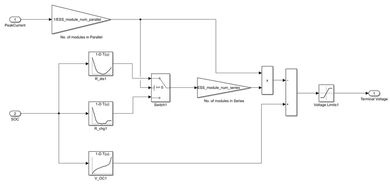
      `V_"batt"=V_"OC"−R_sI_"batt"`
      The above equation is used for the calculation of the terminal voltage. The found SOC is input for three different 1D lookup tables. The internal resistance of discharge and charge, and the open circuit voltage is found using lookup table as SOC as input. The data for comparison is provided in loaded ESS_NiMH6.mat file. The internal resistance found is passed on to the switch where a condition is checked. For the positive current, internal resistance of discharge is used, while for the negative current the internal resistance of charge is used for the `R_s` in the equation. The gain block is used to compensate for 20 different modules, and the terminal voltage is calculated as per the equation.
      
      
      
  • Transmission
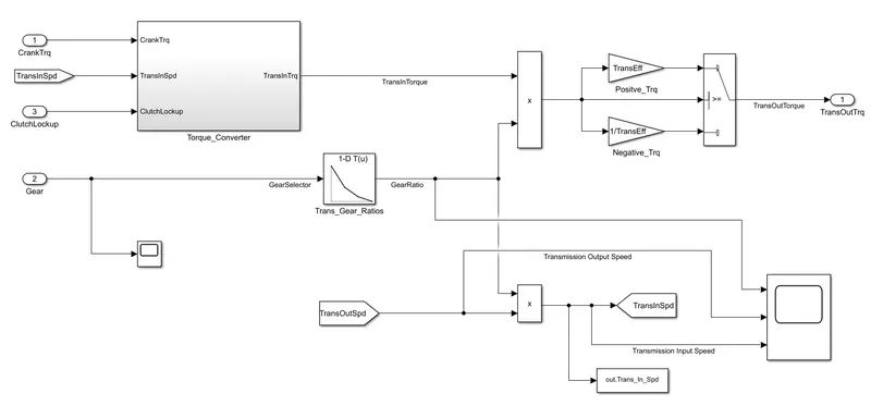    The transmission takes engine torque, gear and additionally the clutch lockup signal as inputs. The signals are then passed into Torque converter. The transmission torque from the torque converter is passed into the gear system where the speed and torque changes as per the gear reduction. The selected gear corresponding to a particular time is used to find the corresponding gear ratio value using the lookup table and is multiplied with torque from the torque converter. The switch is used in order to consider the efficiency of the transmission. The sample output from the scope for the UDDS drive cycle is shown in Figure 10.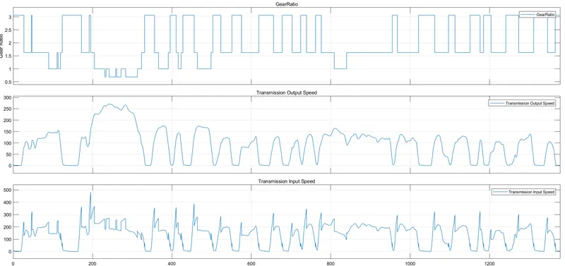
    
    Figure 10: Sample scope output for UDDS drivecycle in the Transmission block.
    
    
    
    • Torque_Converter
      
      
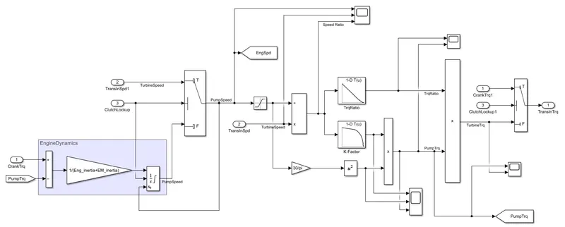
      A torque converter is a form of fluid coupling that transfer rotating power from a vehicle's engine to its transmission. In an automatic transmission, it replaces the mechanical clutch. The pump which is coupled with the engine is used to derive the pump speed and dividing it with the transmission speed gives the speed ratio. This speed ratio is used to find the torque ratio and capacity factor using the lookup table. The capacity factor is used for finding the pump torque from the pump speed using the equation,
      `"Capacity Factor " k_f="pump speed in rpm"/(sqrt"pump torque in Nm")`
      This pump torque is used to find the turbine torque using the torque ratio. Multiple scopes are used to visualize the various parameters. The sample scope outputs are shown in Figure 7 and 8.
      
      
      
  • Differential
    
    
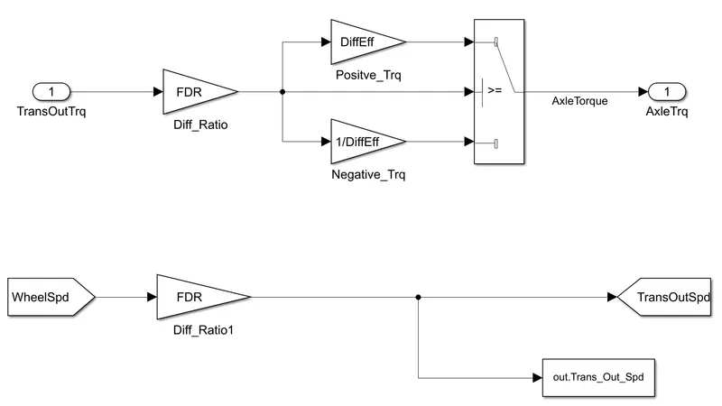
    The Differential subsytem takes the output from the transmission system and reduce it as the gear ratio of the differential. The switch block is used to compensate for the negative and positive sign values. The required parameters are transferred between the other subsytems and the command window using the goto and To Workspace blocks.
    
    
    
  • Wheels
    
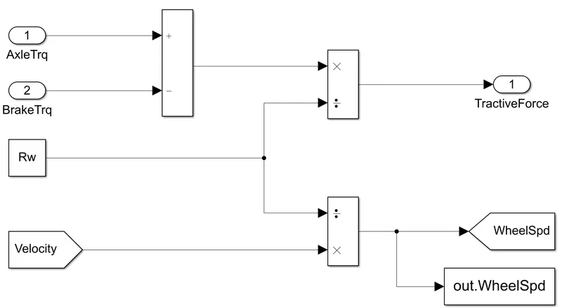
    The Wheels subsystem takes the axle torque and brake torque as the input. The brake torque is to reduce the axle torque to maintain the desired vehicle speed. Dividing the dynamic radius of the wheel with equivalent torque and vehicle velocity gives the tractive force and the wheel speed.
    
    
    
  • Vehicle Dynamics
    
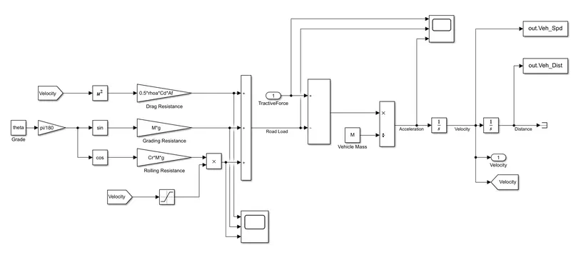
    The Vehicle Dynamics block is used to find the vehicle dynamic characteristics like velocity, acceleration and distance travelled from the tractive force. The vehicle force corresponding to the actual vehicle is the difference between the tractive and the road load. The road load constitutes the drag, rolling and grading resistance. The velocity saturation is multiplied with the rolling resistance to ensure that it is avoided when the vehicle is not in motion. The saturation gives the value 0 for the zero velocity case and 1 for the vehicle with certain velocity. From the equivalent force, the actual vehicle acceleration, velocity and distance travelled can be found. The sample output from the scope for the UDDS drive cycle is shown in Figure 11. The longitudinal dynamics equation which is used for the respective block is,
    `M(dV)/dt=(η_tλ)/R_wT_m−(1/2ρ_aA_fC_d(V±V_w)^2+C_rMgcosθ+Mgsinθ)`
    where, `rho_a` is the air density, `A_f` is the frontal area, `C_d` is the drag coefficient, `V` is the vehicle speed, `V_w` is the wind speed, `C_r` is the rolling resistance coefficient, `M` is the vehicle mass, `g` is the gravity constant and `theta` is the road grade.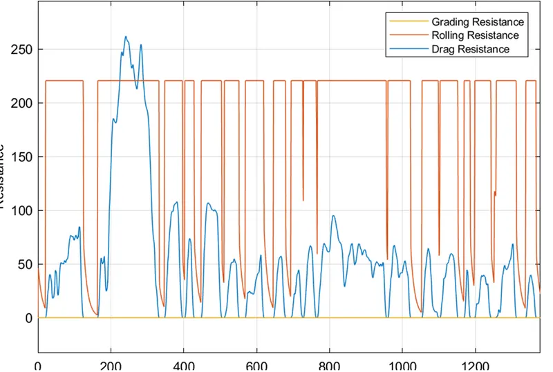
    
    
    Figure 11: Scope output showing various resistance.
    
  
  
  
  
  

MATLAB Post Processing Code:

The MATLAB script "Project2_ProcessingFile" is used to analyze the data from the Simulink model and to generate plots. After the Simulink vehicle model is run, some of the data are sent to the workspace which is used to plot different parameters for the study of conventional vehicle in MATLAB.

%%%%%%%%%%%%%%%%%%%%%%%%%%%%%%%%%%%%%%%%%%%%%%%%%%%%%%%%%%%%%%%%%%%%%
%% Skill-Lync -> Hybrid Drives Development
% Project - Conventional Vehicle Model
% By: Jibin Jafar

% Description:
% The following file is to used with the Initialization file and Simulink
% results for post-processing of the data.

%% Post-Processing File
%  File for post-processing the Conventional vehicle simulation model data

close all;
%% Renaming variables
Time = ans.tout;
Acc_Pdl = ans.Acc_Pdl;          % Accelerator pedal [%]
Brk_Pdl = ans.Brk_Pdl;          % Brake pedal [%]
Trans_In_Spd = ans.Trans_In_Spd*30/pi;  % Transmission input speed [rpm]
Trans_Out_Spd = ans.Trans_Out_Spd*30/pi;% Transmission output speed [rpm]
Eng_Trq = ans.Eng_Trq;          % Engine brake torque [Nm]
Eng_Spd = ans.Eng_Spd*30/pi;    % Engine speed [rpm]
Eng_Fuel_Consump = ans.Eng_Fuel_Consumption;    % Engine fuel consumption [g]
Enf_Fuel_Rate = ans.Eng_Fuel_Rate;  % Engine Fuel COnsumption rate [g/s]
Veh_Dist = ans.Veh_Dist/1000;   % Distance traveled by vehicle [km]
Veh_Spd = ans.Veh_Spd*18/5;     % Vehicle speed [kmph]
WheelSpd = ans.WheelSpd;        % Wheel speed
Gear_Cmd = ans.Gear_Cmd;        % Transmission gear
EM_Spd = ans.EM_Spd*30/pi;      % E Motor speed [rpm]
EM_Trq = ans.EM_Trq;            % E Motor brake torque [Nm]
Ter_Volt = ans.Ter_Volt;        % Pack Terminal VOltage [V]
Current = ans.Current;          % Pack Current [A]
EM_In_Pwr = ans.EM_In_Pwr;      % E Motor Input power [W]
SOC = ans.SOC;                  % Battery state of charge

%% Data Analysis
Eng_Pwr = Eng_Spd.*pi./30.*Eng_Trq./1000;   % Engine brake power [kW]
rho_petrol = 0.7197;                    % Density of petrol [kg/L]
kmpl = Veh_Dist(end)/(Eng_Fuel_Consump(end)/1000/rho_petrol);    % Fuel economy [kmpl] 


%% Plotting vehicle characteristics time trace

% Plot: Transmission Input and Output, Wheel Speed
figure(1)
plot(Time, Trans_In_Spd, 'linewidth', 1, 'Color', 'black');
hold on;
plot(Time, Trans_Out_Spd, 'linewidth', 1, 'Color', 'red');
hold on;
plot(Time, WheelSpd, 'linewidth', 1, 'Color', 'blue');
ylabel('Speed [rpm]');
xlabel('Time [s]');
xlim([0, Time(end)]);
ylim([0, 6000]);
legend('Trans Input','Trans Output','Wheel Speed');
grid on;
grid minor;


% Plot: Engine Torque, Engine Power, Fuel Rate & Fuel Consumption
figure (2)
subplot(4,1,1)
plot(Time, Eng_Trq, 'linewidth', 1, 'Color', 'black');
xlabel('Time [s]');
ylabel('Engine Torque [Nm]');
title('Engine Torque');
grid on;
grid minor;
xlim([0, Time(end)]);

subplot(4,1,2)
plot(Time, Eng_Pwr, 'linewidth', 1, 'Color', 'blue');
xlabel('Time [s]');
ylabel('Engine Power [Nm]');
title('Engine Power');
grid on;
grid minor;
xlim([0, Time(end)]);

subplot(4,1,3)
plot(Time, Enf_Fuel_Rate, 'linewidth', 1, 'Color', 'red');
xlabel('Time [s]');
ylabel('Fuel Rate [g/s]');
title('Engine Fuel Rate');
grid on;
grid minor;
xlim([0, Time(end)]);

subplot(4,1,4)
plot(Time, Eng_Fuel_Consump, 'linewidth', 1, 'Color', 'red');
xlabel('Time [s]');
ylabel('Fuel Consumption [g]');
title('Engine Fuel Consumption');
grid on;
grid minor;
xlim([0, Time(end)]);


% Plot: Accelerator & Brake Pedal, Vehicle actual & desired speed,
% Vehicle DIstance
figure (3)
subplot(3,1,1)
plot(Time, Acc_Pdl, 'linewidth', 1, 'Color', 'black');
hold on;
plot(Time, Brk_Pdl, 'linewidth', 1, 'Color', 'red');
ylabel('Pedal [%]')
xlim([0, Time(end)]);
legend('Accel','Brake');
grid on;
grid minor;

subplot(3,1,2)
hold on;
grid on;
grid minor;
plot(cyc_time, (cyc_vel.*(18./5)),'linewidth', 1,'Color', 'black');
plot(Time, Veh_Spd,':', 'linewidth', 1, 'Color', 'red');
legend('Desired','Actual');
xlim([0, Time(end)]);
xlabel('Time [s]');
ylabel('Velocity [km/h]');

subplot(3,1,3)
plot(Time, Veh_Dist, 'linewidth', 1, 'Color', 'black');
xlim([0, Time(end)]);
xlabel('Time [s]');
ylabel('Distance [km]');
grid on;
grid minor;


% Plot: Engine operating points on engine fuel map
figure('Name','Engine Operating Points');
hold on
grid on
title('Engine Operating Points','fontsize',12);
p1=plot(Eng_map_spd*30/pi,Eng_max_trq,'linewidth',2,'color','r');
p2=line([Eng_map_spd(end)*30/pi Eng_map_spd(end)*30/pi],[0 Eng_max_trq(end)]);
set(p2,'linewidth',1,'linestyle','--','color','k');
p3=line([Eng_map_spd(1)*30/pi Eng_map_spd(1)*30/pi],[0 Eng_max_trq(1)]);
set(p3,'linewidth',1,'linestyle','--','color','k');
[c,h] = contour(Eng_map_spd'*30/pi,Eng_map_trq,Eng_fuel_map');
clabel(c,h);
xlabel('Engine Speed [rpm]');
ylabel('Engine Torque [Nm]');
title('Engine Fuel Consumption Map [g/s]');
p4 = plot(Eng_Spd,Eng_Trq,'.','color','k');
legend([p1 p4],{'Max Curve','Operating Points'});
axis([Eng_map_spd(1)*30/pi Eng_map_spd(end)*30/pi 0 Eng_map_trq(end)]);

% Plot: pack voltage, current and SoC
figure (5)
subplot(3,1,1)
plot(Time, Ter_Volt, 'linewidth', 1, 'Color', 'black');
ylabel('Pack Voltage [V]')
xlim([0, Time(end)]);
grid on;
grid minor;

subplot(3,1,2)
grid on;
grid minor;
plot(Time, Current, 'linewidth', 1, 'Color', 'black');
xlim([0, Time(end)]);
xlabel('Time [s]');
ylabel('Current [A]');
grid on;
grid minor;

subplot(3,1,3)
grid on;
grid minor;
plot(Time, SOC,'linewidth', 1, 'Color', 'black');
xlim([0, Time(end)]);
xlabel('Time [s]');
ylabel('SOC');
grid on;
grid minor;

% Plot: Engine operating points on engine fuel map
figure('Name','Motor Operating Points');
hold on
grid on
title('Motor Operating Points','fontsize',12);
p1=plot(EM_map_spd*30/pi,EM_max_trq,'linewidth',2,'color','r');
p5=plot(EM_map_spd*30/pi,EM_max_gen_trq,'linewidth',2,'color','b');
p2=line([EM_map_spd(end)*30/pi EM_map_spd(end)*30/pi],[0 EM_max_trq(end)]);
set(p2,'linewidth',1,'linestyle','--','color','k');
p3=line([EM_map_spd(1)*30/pi EM_map_spd(1)*30/pi],[0 EM_max_trq(1)]);
set(p3,'linewidth',1,'linestyle','--','color','k');
[c,h] = contour(EM_map_spd'*30/pi,EM_map_trq,EM_inpwr_map');
clabel(c,h);
xlabel('Motor Speed [rpm]');
ylabel('Motor Torque [Nm]');
title('Motor Input Power Map');
p4 = plot(EM_Spd,EM_Trq,'.','color','k');
legend([p1 p4 p5],{'Max Torque Curve','Operating Points','Regen Curve'});
%axis([EM_map_spd(1)*30/pi EM_map_spd(end)*30/pi EM_map_gen_trq(end) EM_map_trq(end)]);
xlim([EM_map_spd(1)*30/pi EM_map_spd(end)*30/pi]);

For the study of the developed vehicle model with various drive cycle, the code to plot the following relations are made:

1. The time trace for engine, transmission input, transmission output and wheel speed on one plot.
2. The engine torque, engine power, fuel rate and fuel consumption using subplots.
3. The accelerator and brake pedal, gear command, vehicle desired and actual speed, vehicle distance using subplots.
4. The engine operating points on the engine fuel map.
5. The motor speed, torque and motor input power using subplots.
6. The battery pack voltage, pack current and SoC using subplots.
7. The motor operating points on the motor input power map, with the motor max motoring and generating torque curves.
   
   

Comparative Study of the Developed Model for UDDS and HWFET Drive Cycle:

	UDDS	HWFET
Fuel Economy Numbers (kmpl) - Only as a Conventional Engine	14.2054	16.5012
Fuel Economy Numbers (kmpl) - As a P1 Hybrid System	14.9598	17.1691

The Hybrid system seemed to have improved fuel economy for both UDDS and HWFET drivecycle. This is because of the involvement of the motor present in the powertrain which provides the torque when necessary.

The fuel economy is seemed to be significantly more for HWFET drive cycle than the UDDS for the same vehicle characteristics. This variation is purely based on drive cycle which is easily observable from Figure 10 and 11. The second subplot in Figure 12 and 13 gives the information on variation of velocity with respect to time. The UDDS drive cycle seems to have more prominent varying velocity over time than HWFET. Therefore, more brake pedal has to be used for UDDS than HWFET which can be observed from the first subplot. The more the brake pedal is pressed, the more will be the energy loss, which in turn means that less will be the fuel economy number.

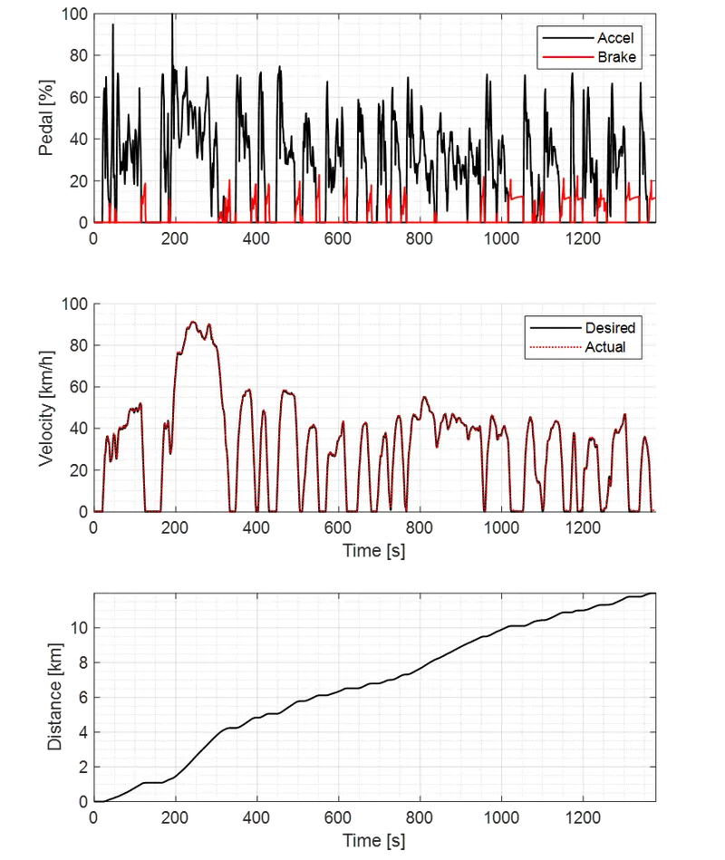
Figure 12: Vehicle Characteristics according to UDDS drive cycle.

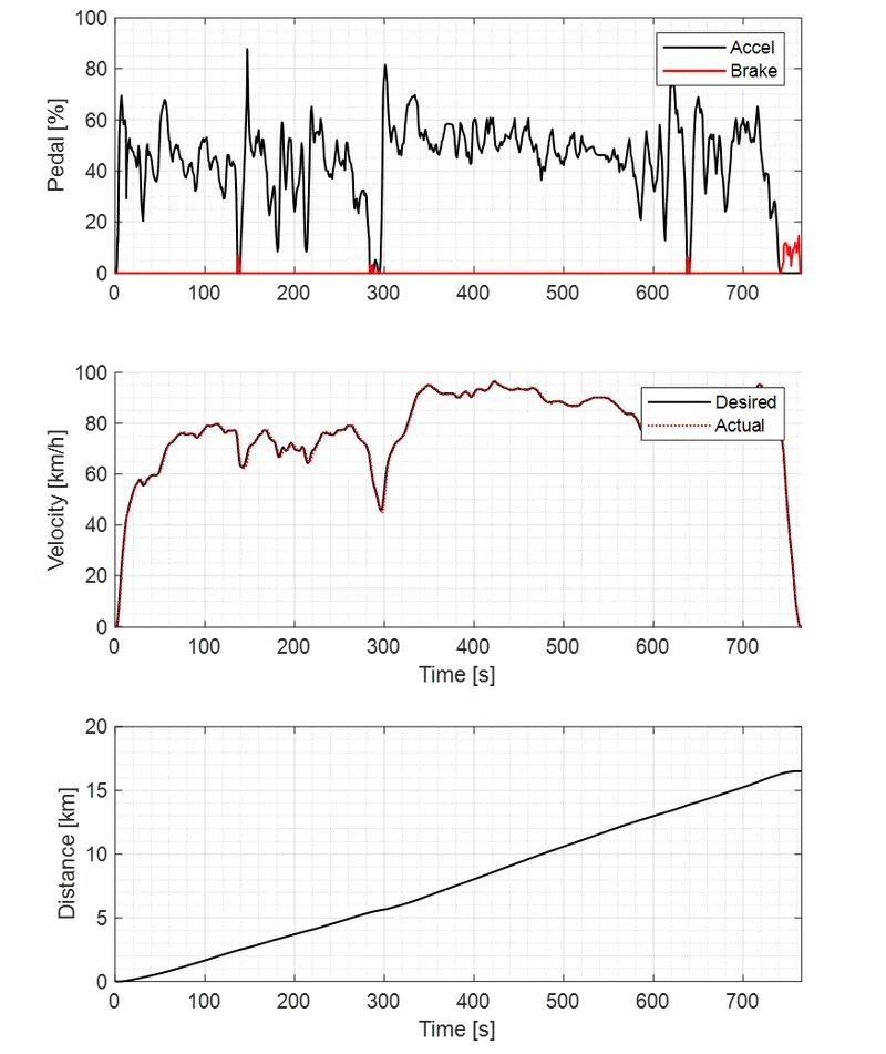
Figure 13: Vehicle Characteristics according to HWFET drive cycle.

From the third subplot, even though the drive cycle duration is significantly less for HWFET than UDDS, the vehicle as per the HWFET seems to have covered way more distance than the other. This is again due to the smoother velocity curve for HWFET. Also, from the subplots three of Figure 12 and 13, it can be seen that the developed model was able to achieve the desired velocity, even though there are minor variations, which is obvious.

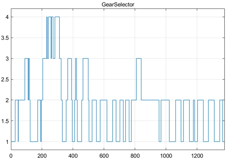
Figure 14: Gear command for UDDS.

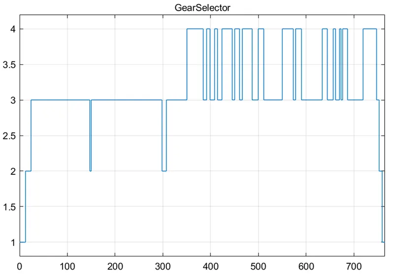
Figure 15: Gear Command for HWFET

The Figure 14 and 15 gives the information on the gear over the entire drive cycle. For the UDDS cycle, more vigorous gear shifting is observed, while for the HWFET, the gear transmission is comparatively smoother.

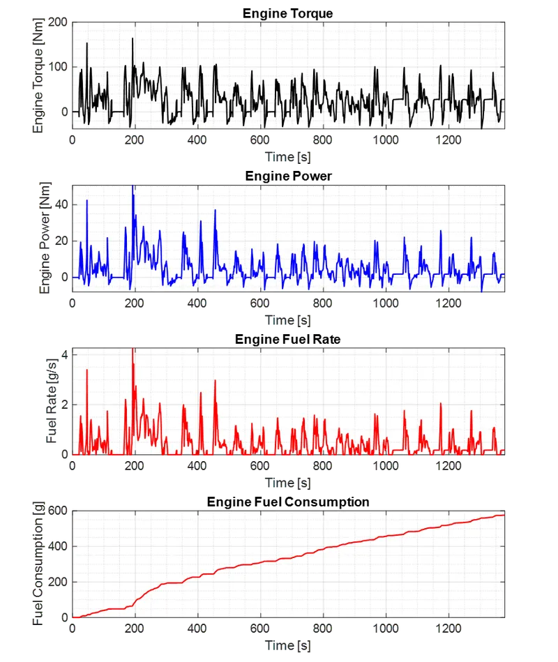
Figure 16: Engine Characteristics according to UDDS drive cycle.

The drive cycle velocity for HWFET is more in the higher range than the UDDS. The power requirement is directly proportional to the power of three for the aerodynamic drag and directly proportional to the rolling and grading resistance. Since, the proportion of higher velocity is more predominant in HWFET, the vehicle requires more power to run HWFET than UDDS, which means that, the fuel consumption of UDDS is less than HWFET even though the drive cycle time is more for UDDS. This can be seen in Figure 16 and 17 in subplot four. The engine torque, engine power and engine fuel rate are seemed to be directly proportional to each other from the Figures.

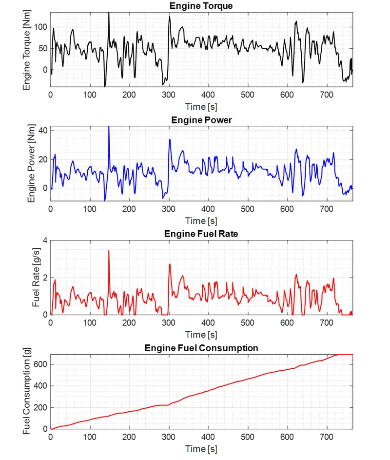
Figure 17: Engine Characteristics according to HWFET drive cycle.

The engine operating points on the engine fuel map is shown in Figure 18 and 19 for UDDS and HWFET drive cycles.

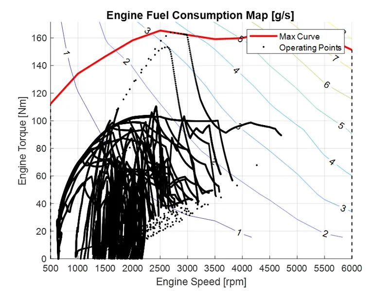
Figure 18: Engine fuel consumption map for UDDS cycle.

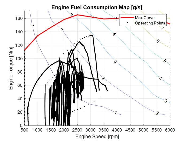
Figure 19: Engine fuel consumption map for HWFET cycle.

From the Figures 18 and 19, the operating points are seemed to be extreme for UDDS drive cycle. These figures reveal that, the engine is capable of going in higher velocity than required in both drive cycle as the max engine speed possible is 6000 rpm. For the cases where the operating parameters are beyond the engine maximum torque curve, the motor can be used to provide additional torque. For HWFET, there is not operating points that is challenging the engine capability, which is not same for UDDS cycle.

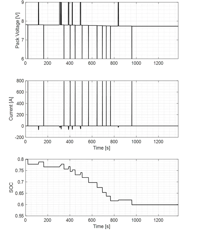
Figure 20: Battery Characteristics for UDDS cycle.

The Figures 20 and 21 shows the Battery characteristics for UDDS and HWFET cycle. Since the HWFET drive cycle doesn't require high torques (seen from Figure 19) and with less velocity variation (seen from Figure 13), the motor usage is very less, thereby the battery usage is less. The charge present in the Battery is initially used for starting the engine later which is only charged (refer Figure 21, subplot 3). But for the UDDS drive cycle, it is totally different. Due to the high torque requirement (Figure 18) and sudden velocity variations (Figure 12), the motor is used so often taking charge from the battery. The state of charge (Figure 20, subplot 3) shows that charge content in keep on decreasing even though minute recharging can be seen. The battery here in this cycle reaches the allowed minimum SOC of 0.6, which is due to the aggressiveness of the drive cycle.

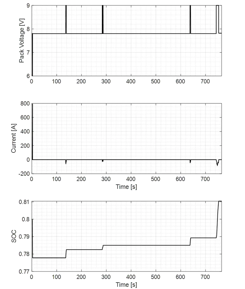
Figure 21: Battery Characteristics for HWFET cycle.

The vehicle operating points on the motor power map is shown in Figure 22 and 23 for UDDS and HWFET drive cycles.

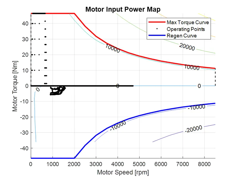
Figure 22: Electric Motor Input Power Map for UDDS.

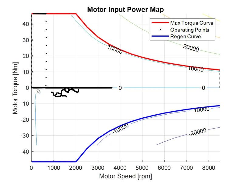
Figure 23: Electric Motor Input Power Map for HWFET.

The operating points on the motor curve is mostly zero torque values compared to that of operating points on engine fuel map. This is because of the P1 construction of hybrid system. All the points are seemed to be within the motor limits.

Downloadable Link:

The developed MATLAB programs and Simulink model can be downloaded from:
https://drive.google.com/drive/folders/1A7HX4a8gdGnsekTinYAQMUJu_VFFn-jh?usp=sharing

Conclusion:

The MATLAB script for both initializing and post processing has be successfully made, and a forward energy-based fuel consumption Simulink model of a P1 Hybrid vehicle is also developed successfully, and the functionality is checked. The comparative study of UDDS and HWFET for the developed vehicle model is analyzed.