Project 2

Drive Cycles:

A driving cycle is a series of data points representing the speed of a vehicle versus time. Driving cycles are produced by different countries and organizations to assess the performance of vehicles in various ways, as for instance fuel consumption, electric vehicle autonomy and polluting emissions. Fuel consumption and emission tests are performed on chassis dynamometers. Tailpipe emissions are collected and measured to indicate the performance of the vehicle.

Another use for driving cycles is in vehicle simulations. More specifically, they are used in propulsion system simulations to predict performance of internal combustion engines, transmissions, electric drive systems, batteries, fuel cell systems, and similar components. Some driving cycles are derived theoretically, as it is preferred in the European Union, whereas others are direct measurements of a driving pattern deemed representative.

Most commom drive cycles:

• WLTC
• NEDC
• SORDS
• FTP-75
• UDDS
• HWFET

UDDS:

UDDS stands for Urban Dynamometer Driving Schedule, and refers to a United States Environmental Protection Agency mandated dynamometer test on fuel economy that represents city driving conditions which is used for light duty vehicle testing. It is also known as U.S. FTP-72 (Federal Test Procedure) cycle, LA-4 cycle, in Sweden as A10 or CVS (Constant Volume Sampler) cycle and in Australia as the ADR 27 (Australian Design Rules) cycle.

Though it was originally created as a reference point for fossil fueled vehicles, it is also used to give estimates on how many miles an electric vehicle will travel on a single charge.

HWFET:

The Highway Fuel Economy Test (HWFET or HFET) cycle is a chassis dynamometer driving schedule developed by the US EPA for the determination of fuel economy of light duty vehicles. The HWFET is used to determine the highway fuel economy rating, while the city rating is based on the FTP-75 test.

Code:

The below code is to determine the variable which is extracted from the simulink model using 'to workspace' command and also for plotting the desired values. We can change the drive cycle to get a result for various drive cycle by using the same code.

Code to select Drive cycle:

%% Vehicle Parameters
M = 1500;       % Vehicle weight [kg]
Cr = 0.015;     % Rolling resistance coefficient
Rw = 0.35;      % Rolling radius [m]
Cd = 0.33;      % Drag coefficient 
Af = 2;         % Frontal area [m2]
rhoa = 1.225;   % Air density [kg/m3]
Vwind = 0;      % Wind velocity [kmph]
g = 9.81;       % Gravitational acceleration [m/s2]
theta = 0;      % Slope [deg]
myu_road_tire = 1; % Coefficient of friction between tire - road interface

%% Powertrain Parameters 
FDR = 3.73;                         % Final Drive Ratio / Diff Ratio
DiffEff = 0.99;                     % Differential efficiency (assumed independent of operating conditions)

NumGear = 4;                        % Number of gears in transmission
TransGear = [1:NumGear];            % Transmission Gears
TransRatio = [3.06, 1.62, 1, 0.7];  % Corresponding Transmission ratios
TransEff = 0.90;                    % Transmission efficiency (assumed independent of operating conditions)

TC_SR = [0, .5, .6, .7, .8, .87, .92, .94, .96, .97, 1];   % Torque Converter Speed Ratio (Matlab default) -> TurbSpd/PumpSpd  
TC_TR = [2.232, 1.5462, 1.4058, 1.2746, 1.1528, 1.0732, 1.0192, 1, 1, 1, 1];   % Torque Converter Torque Ratio (Matlab default) -> TurbTrq/PumpTrq
TC_Cf = 1e-4 * [.72558, .66322, .63463, .59042, .51331, .4144, .29287, .22444, .12186, .04386, 0]; % Torque Converter Capacity Factor (Matlab default) -> PumpTrq/PumpSpd^2 [Nm/rpm^2]

load Vehicle_Data/Engine_data_1_9L_Saturn_95kW
load Vehicle_Data/Trans_Shift_map
load Vehicle_Data/EM_Honda_Insight_10kW
load Vehicle_Data/ESS_NiMH6


ESS_init_soc = 0.8;
ESS_soc_max = 0.9;
ESS_soc_min = 0.6;


%% Driver Parameters
Kp = 10;                    % P gain for driver PI model
Ki = 1;                     % I gain for driver PI model
Drive_Cycle_Select = 1;     % Drive cycle selection

% Drive cycle values in m/s

if Drive_Cycle_Select == 1
    load DriveCycles/UDDS;
    
elseif Drive_Cycle_Select == 2
    load DriveCycles/HWFET;
    
elseif Drive_Cycle_Select == 3
    load DriveCycles/FTP;
    
elseif Drive_Cycle_Select == 4
    load DriveCycles/US06;
    
elseif Drive_Cycle_Select == 5
    load DriveCycles/NEDC;
    
elseif Drive_Cycle_Select == 6
    load DriveCycles/WLTP;
 
end

time_end = cyc_time(end);
vel_end = cyc_vel(end);

Main coding:

%% Renaming variables
Time = out.tout;
Acc_Pdl = out.Acc_Pdl;          % Accelerator pedal [%]
Brk_Pdl = out.Brk_Pdl;          % Brake pedal [%]
Gear_Cmd = out.Gear_Cmd;        % Transmission gear
Trans_In_Spd = out.Trans_In_Spd*30/pi;  % Transmission input speed [rpm]
Trans_Out_Spd = out.Trans_Out_Spd*30/pi;% Transmission output speed [rpm]
Eng_Trq = out.Eng_Trq;          % Engine brake torque [Nm]
Eng_Spd = out.Eng_Spd*30/pi;    % Engine speed [rpm]
Eng_Fuel_Consump = out.Eng_Fuel_Consumption;    % Engine fuel consumption [g]
Veh_Dist = out.Veh_Dist/1000;   % Distance traveled by vehicle [km]
Veh_Spd = out.Veh_Spd*18/5;     % Vehicle speed [kmph]
Eng_Fuel_rate = out.Eng_Fuel_Rate;
Wheel_Speed = out.Wheel_Speed;
soc = out.soc*100;
PackCurrent = out.PackCurrent;
Voltage = out.Voltage;
EM_out_Pwr = out.ElecPwr;
EMTrq = out.EMTrq;
%% Data Analysis
Eng_Pwr = Eng_Spd.*pi/30.*Eng_Trq/1000;   % Engine brake power [kW]
EM_in_Pwr = Eng_Spd.*pi/30.*EMTrq/1000;   %Electric motor power 
rho_petrol = 0.7197;                    % Density of petrol [kg/L]
%kmpl = Veh_Dist(end)/(Eng_Fuel_Consump(end)/1000/rho_petrol);    % Fuel economy [kmpl] 
%kmpl1 = Veh_Dist(end)/(EM_in_Pwr(end)/100); 

%% Plotting vehicle characteristics time trace
figure(1)
subplot(3,1,1)
title('For HWFET drive')
hold on
grid on
plot(Time, Acc_Pdl, 'linewidth', 1, 'Color', 'blue');
plot(Time, Brk_Pdl, 'linewidth', 1, 'Color', 'red');
ylabel('Pedal [%]')
xlim([0, Time(end)]);
legend('Accel','Brake');
subplot(3,1,2)
hold on
grid on
plot(Time, Trans_In_Spd, 'linewidth', 1, 'Color', 'blue');
plot(Time, Trans_Out_Spd, 'linewidth', 1, 'Color', 'red');
ylabel('Speed [rpm]')
xlim([0, Time(end)]);
title('For UDDS drive')
ylim([0, 6000]);
legend('Trans Input','Trans Output');
subplot(3,1,3)
hold on
grid on
plot(Time, Gear_Cmd, 'linewidth', 1, 'Color', 'black');
xlim([0, Time(end)]);
xlabel('Time [s]');
ylabel('Gear');
title('For UDDS drive')

%% Plotting engine operating points on engine fuel map
figure('Name','Engine Operating Points');
hold on
grid on
title('Engine Operating Points','fontsize',12);
p1=plot(Eng_map_spd*30/pi,Eng_max_trq,'linewidth',1,'color','r');
p2=line([Eng_map_spd(end)*30/pi Eng_map_spd(end)*30/pi],[0 Eng_max_trq(end)]);
set(p2,'linewidth',1,'linestyle','--','color','k');
p3=line([Eng_map_spd(1)*30/pi Eng_map_spd(1)*30/pi],[0 Eng_max_trq(1)]);
set(p3,'linewidth',1,'linestyle','--','color','k');
[c,h] = contour(Eng_map_spd*30/pi,Eng_map_trq,Eng_fuel_map');
clabel(c,h);
xlabel('Engine Speed [rpm]');
ylabel('Engine Torque [Nm]');
title('Engine Fuel Consumption Map [g/s]  for UDDS Drive');
%p4 = plot(Eng_Spd,Eng_Trq,'color','g');
legend([p1 p3],{'Max Curve','Operating Points'});
axis([Eng_map_spd(1)*30/pi Eng_map_spd(end)*30/pi 0 Eng_map_trq(end)]);

figure(3)
hold on
plot(Veh_Dist,kmpl1)
xlabel('Distance in Km')
ylabel('Fuel consumption in L')
title('Fuel consumption for UDDS')

disp('            Fuel economy numbers')
disp('           ********************') 
disp('Drive cycle                 kmpl')
fprintf('\n')
fprintf('UDDS                   %d\n',kmpl1)
%fprintf('HWFET                 %d\n',kmpl2)

figure(4)
subplot(4,1,1)
title('For UDDS drive')
hold on
grid on
plot(Time,Eng_Pwr, 'linewidth', 1, 'Color', 'blue');
xlabel('Time')
ylabel('KW')
xlim([0, Time(end)]);
legend('Power');
subplot(4,1,2)
hold on
grid on
plot(Time, Eng_Trq, 'linewidth', 1, 'Color', 'red');
xlabel('Time')
ylabel('Nm')
xlim([0, Time(end)]);
legend('Torque');
subplot(4,1,3)
hold on
grid on
plot(Time, Eng_Fuel_Consump, 'linewidth', 1, 'Color', 'blue');
xlabel('Time')
ylabel('g')
xlim([0, Time(end)]);
legend('Fuel Consumption');
subplot(4,1,4)
hold on
grid on
plot(Time, Eng_Fuel_rate, 'linewidth', 1, 'Color', 'red');
xlabel('Time')
ylabel('g')
xlim([0, Time(end)]);
legend('Engine Fuel Rate');

figure(5)
subplot(3,1,1)
title('For UDDS drive')
hold on
grid on
plot(Time,Trans_In_Spd, 'linewidth', 1, 'Color', 'blue');
xlabel('Time')
ylabel('Rpm')
xlim([0, Time(end)]);
legend('Input Transmission ');
subplot(3,1,2)
hold on
grid on
plot(Time, Trans_Out_Spd, 'linewidth', 1, 'Color', 'red');
xlabel('Time')
ylabel('Rpm')
xlim([0, Time(end)]);
legend('Output Transmission');
subplot(3,1,3)
hold on
grid on
plot(Time, Wheel_Speed, 'linewidth', 1, 'Color', 'g');
xlabel('Time')
ylabel('m/min')
xlim([0, Time(end)]);
legend('Wheel Speed');


figure(6)
subplot(3,1,1)
title('For HWFET drive')
hold on
grid on
plot(Time,Eng_Spd, 'linewidth', 1, 'Color', 'blue');
xlabel('Time')
ylabel('Rpm')
xlim([0, Time(end)]);
legend('Electic motor speed ');
subplot(3,1,2)
hold on
grid on
plot(Time, EMTrq, 'linewidth', 1, 'Color', 'red');
xlabel('Time')
ylabel('Nm')
xlim([0, Time(end)]);
legend('Electic motor Torque');
subplot(3,1,3)
hold on
grid on
plot(Time, EM_in_Pwr, 'linewidth', 1, 'Color', 'g');
xlabel('Time')
ylabel('KW')
xlim([0, Time(end)]);
legend('Electric motor power');

figure(7)
subplot(3,1,1)
title('For HWFET drive')
hold on
grid on
plot(Time,PackCurrent, 'linewidth', 1, 'Color', 'blue');
xlabel('Time')
ylabel('Ah')
xlim([0, Time(end)]);
legend('Pack current ');
subplot(3,1,2)
hold on
grid on
plot(Time, Voltage, 'linewidth', 1, 'Color', 'red');
xlabel('Time')
ylabel('V')
xlim([0, Time(end)]);
legend('Voltage');
subplot(3,1,3)
hold on
grid on
plot(Time, soc, 'linewidth', 1, 'Color', 'g');
xlabel('Time')
ylabel('[%]')
xlim([0, Time(end)]);
legend('State of current');

figure('Name','Engine Operating Points');
hold on
grid on
title('Engine Operating Points','fontsize',12);
p1=plot(EM_map_spd*30/pi,EM_max_trq,'linewidth',1,'color','r');
p2=line([EM_map_spd(end)*30/pi EM_map_spd(end)*30/pi],[0 EM_max_trq(end)]);
set(p2,'linewidth',1,'linestyle',':','color','k');
p3=line([EM_map_spd(1)*30/pi EM_map_spd(1)*30/pi],[0 EM_max_trq(1)]);
set(p3,'linewidth',1,'linestyle',':','color','k');
[c,h] = contour(EM_map_spd*30/pi,EM_map_trq,EM_inpwr_map');
clabel(c,h);
xlabel('EM Speed [rpm]');
ylabel('EM Torque [Nm]');
title('Motor input power Map');
p4 = plot(Eng_Spd,EMTrq,'color','r');
legend([p1 p4],{'Max Curve','Operating Points'});
axis([EM_map_spd(1)*30/pi EM_map_spd(end)*30/pi 0 EM_map_trq(end)]);
ylim([-70,70]);

Simulink Model :

Vehicle model

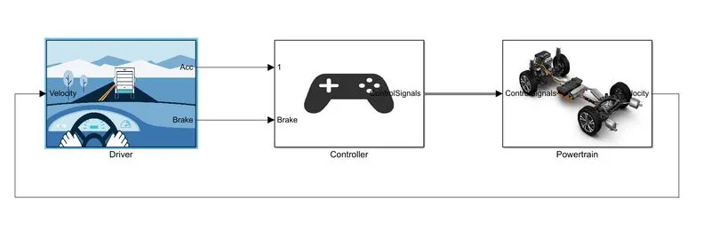
The vehicle has a three major blocks

1. Driver
2. Controller
3. Powertrain

1.Driver

The driver in other words the user has a various inputs like brake,accelerator,gear and etc. in various situation. There is a standard drive modes are available for various drive modes.

• UDDS
• HWFET
• FTP
• US06
• NEDC
• WLTP

Here we will see only UDDS and HWFET drive cycles only.

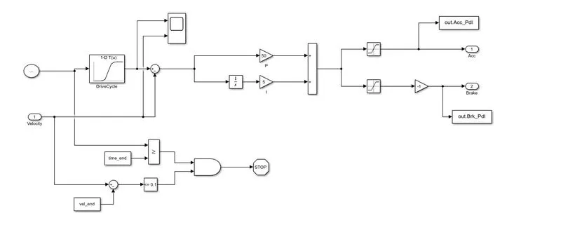
The driver block take input as a drive cycle, based on that drive cycle datas it simulates the cycle to get a desired output.

And it has a seperate circuit to cutoff the engine when the cycle gets over.

2.Controller

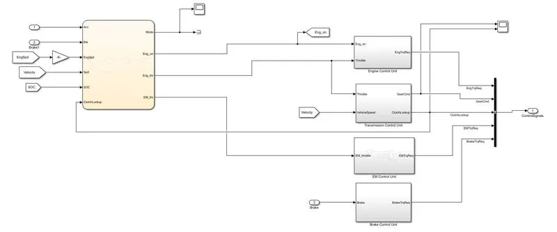
The above image repereset the elements of controller unit which consists of state flow chart and other control unit. The state flow chart is given below

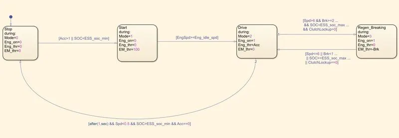
The chart took input as accelerator,break,state of current and clutch and gives output as Engine on, engine off,engine throttle,electric motor throttle and mode

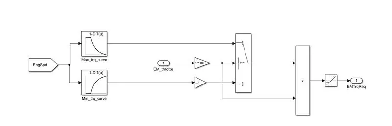
The electric motor control unit is given below which convertes the speed into torque

3.Powertrain

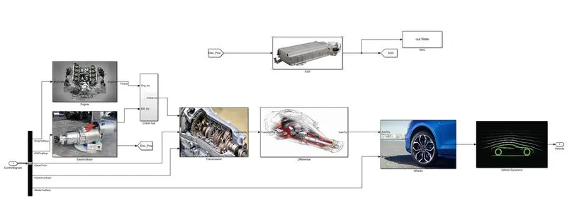
The power train block that incles of Engine,Electric motor, Tranmission, Differencial, Wheels and vehicle dynamics.

i.Engine

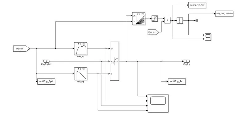
The engine block useing lookuptable to feed the maximum and minimum torque datas. By using these datas it convertes it into torque and gives the fuel consumption detailes .

ii.Electric motor

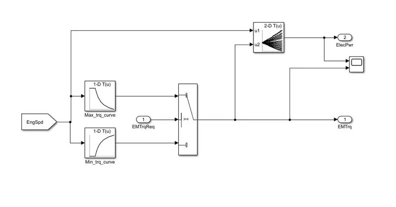
The lookup table

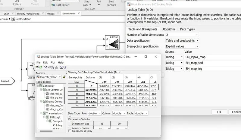
The above image shows the parameters used in the lookup table which is used to get electrical power output.

ESS(Energy storage system):

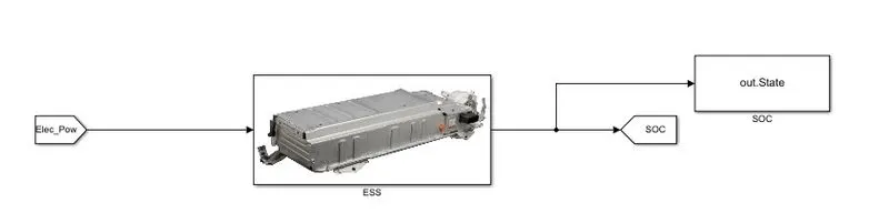
The above model represent the basic layout for the battery which consist of energy storage system and output as a state of current. The energy storage sub system has a layout as follows

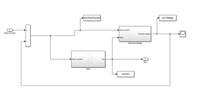
As we can see in the above diagram it consist a pair of subsystem which is State of current and Terminal voltage. And it has three outputs which feed the data to the workspace, for that 'To workspace' command was used.

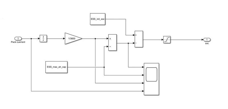
The above system show the elements for the State of current(SOC) sub system

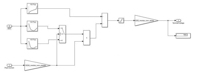
Finally the Terminal voltage sub system as shown above, it has a input for charging and also discharging. For that the 2D looktable used to feed the data.

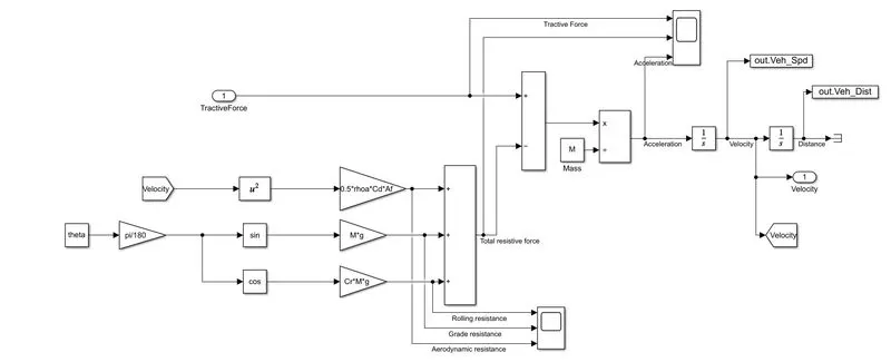
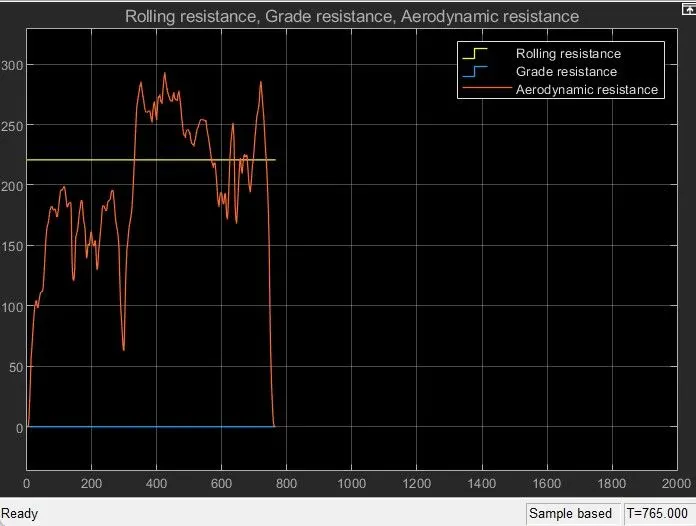
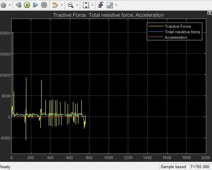
The above block repesent the vehicle dynamics block which is basically to calculate the vehicle acceleration, velocity and distance. The vehicle acceleration calculated from the sum of tractive force and total resistance force. The resistance force consists of Rolling, Grade and aerodynamic resistance. The below graph show how these resistance act on a vehicle

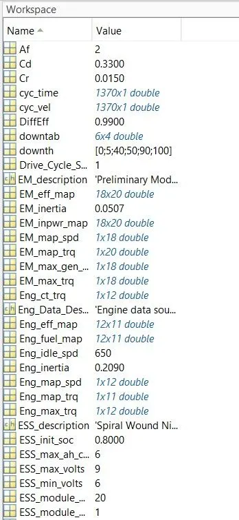
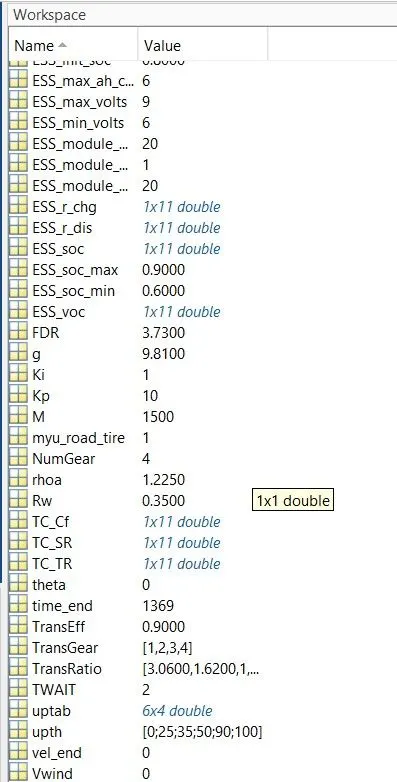
The parameters which stored in matlab workspace is shown below:

Results:

Drive cycle	Km/unit(W)
UDDS	3.082586e+02
HWFET	4.243316e+02

Plots:

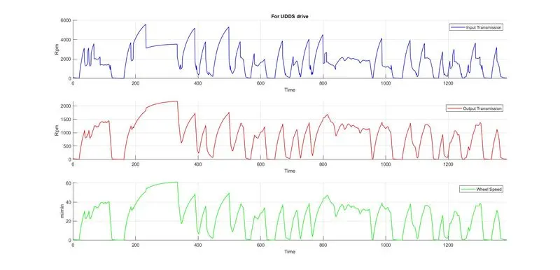
The time trace for engine, transmission input, transmission output and wheel speed.

For UDDS cycle

For HWFET cycle

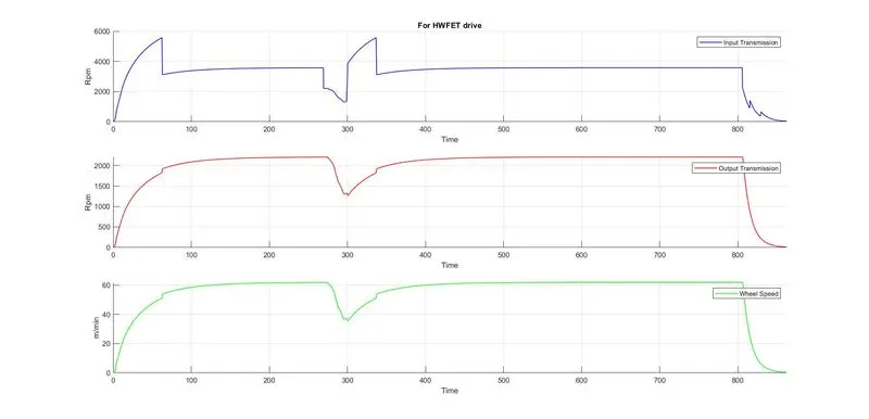
• The above plots were plotted for transmission input,transmission output and wheel speed with respect to time for both UDDS and HWFET drive cycles.
• The input transmission got from the engine and it varies depend on the driver input, but here by using UDDS drive cycle the inputs were already defined.
• So the input transmission plot shows how the input goes.
• Then the output transmission and wheel speed act depend upon the input transmission.
• We can see that the wheel speed and output transmission curves were goes same to each other, because that two variables were react same as each other.

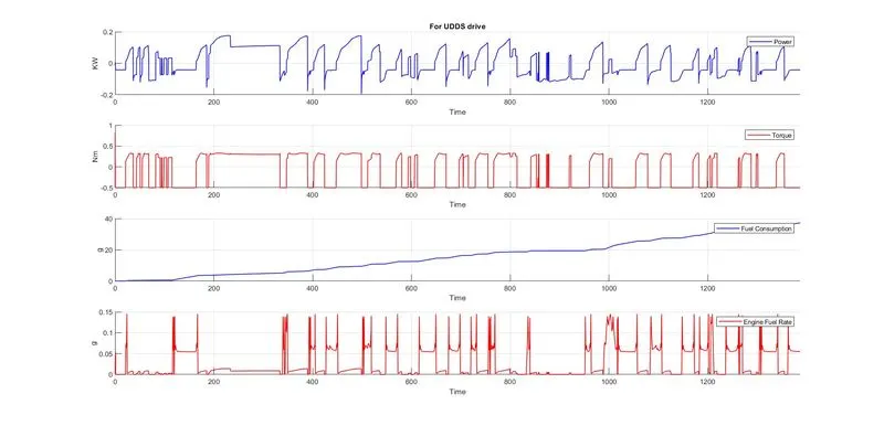
Engine torque,power and fuel rate,consumption plots

For UDDS drive cycle

For HWFET drive cycle

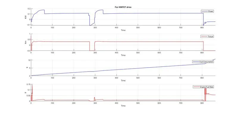
• The above plot shows the Engine power,engine torque,fuel rate and fuel consumption curves over time.
• We can see that the power and torque curves goes like same because these two factors dependes on each other.
• The other two curves represent the engine fuel consumption and engine fuel rate values.
• The fuel consumption and fuel rate is in grams as y axis.
• The fuel consumption shows the over all fuel consume over the time period.
• The fuel rate shows the fuel coumption of an engine at the particular time, so it varies over the time period.

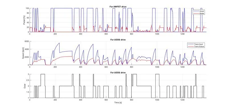
Plot for accelerator and break pedal,gear command,vehicle desired and actual speed

For UDDS drive cycle

For HWFET drive cycle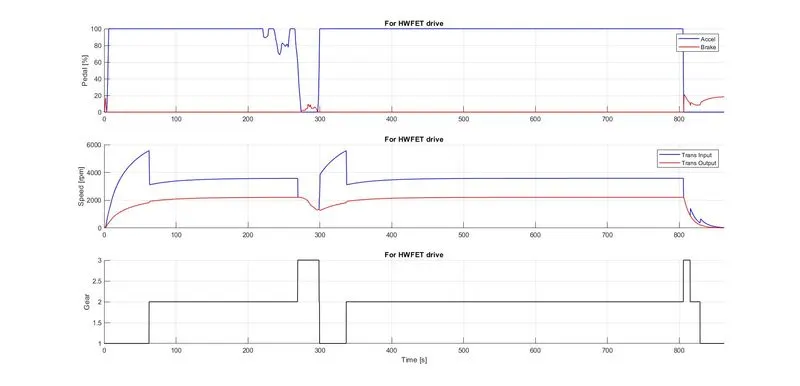

• The above plot consists of three plots which is accelerator and brake pedal, vehicle desired and actual speed and gear command
• The first plot has two curves, the blue one reperesent accelerator behavior and the red one reperesant the breake behavior.
• When the brake curve raises the accelerator cuves goes down which shows these two curves inversly proposnal.
• The second curve shows the vehicle desired and actual speed.
• The input transmission goes quick vertical manner becaues it get from the user but the output won't, because it depends on the vehicle behavier.
• The third plot shows the gear command from the user.
• The lower gear basically has high torque and low power which means it can pull heavy weigh but it can't go high speed.
• But similarly the higher gear has low torque and high power.

Contour plot for engine fuel map

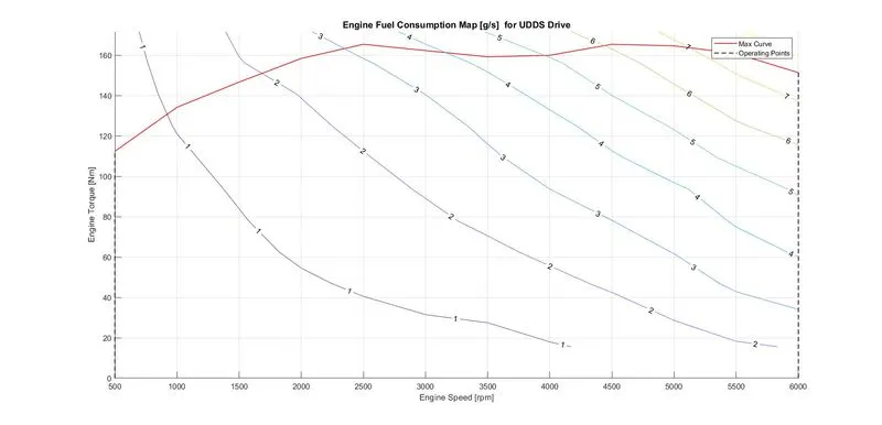
• The above map build by using contour command.
• The contour command basically has the inputs, it has x,y and z axis.
• The z axis is a 3D plot which shows top view of the plot we can also say that cross section view.
• The red line reperesent the maximum torque curve.
• The dotted lines reperesent the engine operating points where the engine operates randomly.
• The z axis which used here is engine fuel map.

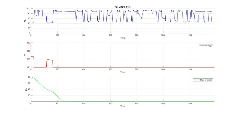
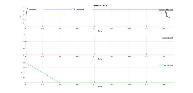
Plot for pack voltage, current and SoC

For UDDS drive cycle

For HWFET drive cycle

Contour plot for motor input power map

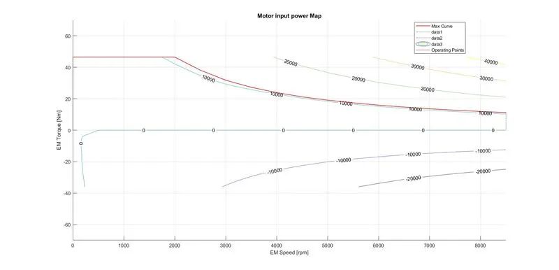
• The above map build by using contour command.
• The contour command basically has the inputs, it has x,y and z axis.
• The z axis is a 3D plot which shows top view of the plot we can also say that cross section view.
• The red line reperesent the maximum torque curve.
• The dotted lines reperesent the engine operating points where the engine operates randomly.
• The z axis which used here is Electric motor input power.

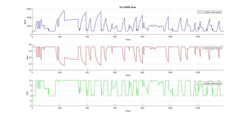
Plot for motor speed, torque, motor input power

For UDDS drive cycle

For HWFET drive cycle

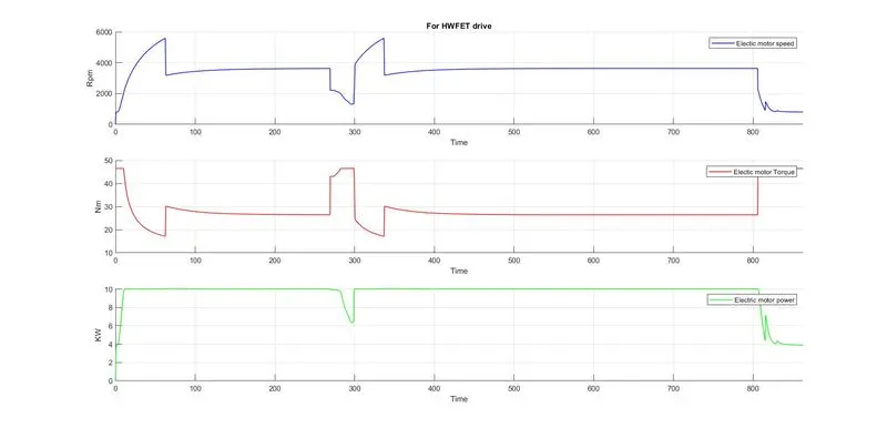
• The above plots were plotted for Electric motor speed,electric motor torque and electric motor power with respect to time for both UDDS and HWFET drive cycles.
• The Electric motor speed got from the electric motor subsystem and it varies depend on the driver input, but here by using UDDS drive cycle the inputs were already defined.
• We can see that the power and torque curves goes like same because these two factors dependes on each other(inversely proportional).
• The electric motor power is based on the two factors which is motor speed and torque

Conclution:

The above report is basically to explain the engine and elecric motor behaviors over the time period with various operating conditions. And the Drive cycles are the standard operating condition which helps to analyse the engine performance. Every engine manufactureres used these drive cycles to analyze engine performance which helps them to know how the engine produce output.