Project 2 - Rankine cycle Simulator
Aim : Create a Rankine Cycle Simulator using OCTAVE/MATLAB
Objective
- To calculate the state points of the Rankine Cycle based on user inputs.
- Extract the datas from the XSteam file provided.
- To calculate the parameters in all points
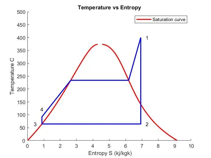
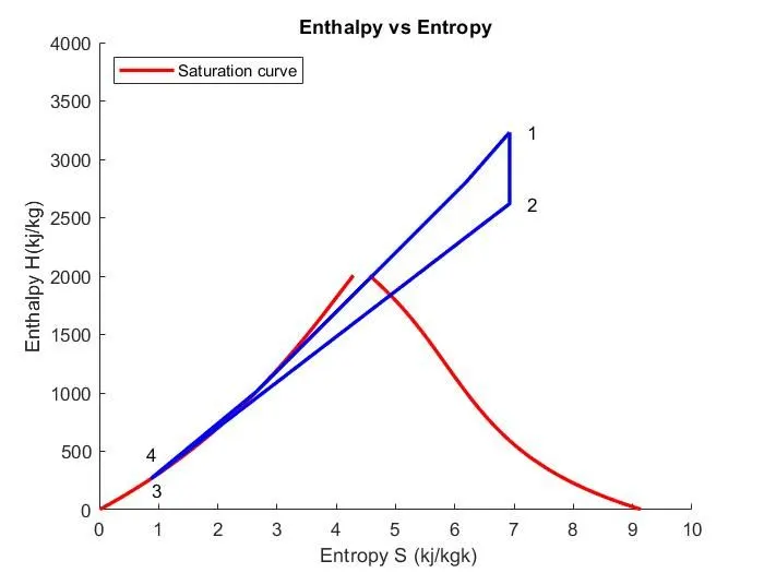
- To plot the corresponding T-s and h-s plots for the given set of inputs.
Rankine Cycle
The Rankine cycle closely describes the process by which steam engines commonly found in thermal power generation plants harness the thermal energy of a fuel or other heat source to generate electricity. Possible heat sources include combustion of fossil fuels such as coal, natural gas, or oil, renewable fuels like biomass or ethanol, nuclear fission, and concentrated solar power. Common heat sinks include ambient air above or around a facility and bodies of water such as rivers, ponds, and oceans.
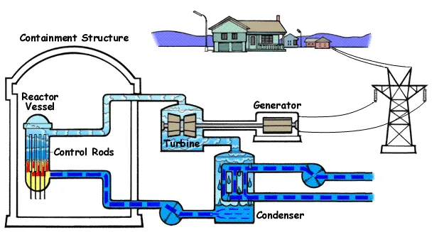
- Process 1–2: The working fluid is pumped from low to high pressure. As the fluid is a liquid at this stage, the pump requires little input energy. Process 1-2 is isentropic compression.
- Process 2–3: The high-pressure liquid enters a boiler, where it is heated at constant pressure by an external heat source to become a dry saturated vapour. The input energy required can be easily calculated graphically, using an enthalpy entropy chart , or numerically, using software. Process 2-3 is constant pressure heat addition in boiler.
- Process 3–4: The dry saturated vapour expands through a turbine, generating power. This decreases the temperature and pressure of the vapour, and some condensation may occur. The output in this process can be easily calculated using the chart or tables noted above. Process 3-4 is isentropic expansion.
- Process 4–1: The wet vapour then enters a condenser, where it is condensed at a constant pressure to become a saturated liquid. Process 4-1 is constant pressure heat rejection in condenser.
Code:
clear all
close all
clc

%statements
fprintf('                                           RANKINE CYCLE SIMULATOR   \n\n ')
fprintf('1-2 is Isentropic  Expansion in the turbine \n')
fprintf('2-3 is constant pressure heat rejection by the condenser\n')
fprintf('3-4 is Isentropic compression in the pump\n')
fprintf('4-1 is constant pressure heat addition by the boiler\n\n')

%inputs getting from user
p1 = input('Enter the pressure value at the Turbine inlet (bar) : ') ;
t1 = input('Enter the temperature value at the Turbine inlet (degree celcius) : ') ;
p2 = input('Enter the pressure at the Condenser (bar) : ') ;
fprintf('\n');
fprintf('                                                     RESULTS\n')

%inpts
h1 = XSteam('h_pT',p1,t1);
s1 = XSteam('s_pT',p1,t1);

%State point 2
%calculation
s2 = s1;                                                          %Iscentropic expansion
sl2 = XSteam('sL_p',p2);
sg2 = XSteam('sV_p',p2);
g = 1.4;                                                          %gama
%by using iscentropic expansion equation
t2 = t1*((p2/p1)^(1-(1/g)));
h2 = XSteam('h_pt',p2,t2);
x2 = (s2-sl2)/(sg2-sl2);

%State point 3
%Constant pressure heat removal
p3 = p2;
t3 = t2;
s3 = XSteam('sL_T',t3);
h3 = XSteam('hL_T',t3);

%State point 4
s4 = s3;
p4 = p1;
cp4 = XSteam('Cp_ps',p4,s4);
cv4 = XSteam('Cv_ps',p4,s4);
g = (cp4/cv4);
t4 = (t3*((p3/p4)^((1-g)/g)));

%work done by turbine
Wturbine = h1-h2;

%work done by pump
v3 = XSteam('vL_p',p3);
Wpump = v3*(p4-p3)*100;

%net work
Wnet = Wturbine - Wpump;

%Specific steam consumpsion
ssc = (3600/Wnet);

%Efficiency
h4 = h3+Wpump;
Qin = h1-h4;
efficiency = ((Wturbine-Wpump)/Qin)*100;

%calcuating H,S and T for Steam at the liquid, wet ,dry and super heated
%states
t6 = XSteam('Tsat_p',p1);
t5 = t6;
s5 = XSteam('sL_p',p1);
s6 = XSteam('sV_p',p1);
h5 = XSteam('hL_p',p1);
h6 = XSteam('hV_p',p1);

%To plot saturated curve
T= linspace (0,400,500);
for i = 1:length(T)
    sl(i) = XSteam('sL_T',T(i));
    sg(i) = XSteam('sV_T',T(i));
    hl(i) = XSteam('hL_T',T(i));
    hg(i) = XSteam('hV_T',T(i));
end

%plotting TS
figure(1)
hold on
plot(sl,T,'r','linewidth',2)
plot(sg,T,'color','r','linewidth',2)
plot([s1 s2 s3 s4 s5 s6 s1],[t1 t2 t3 t4 t5 t6 t1],'b','linewidth',2)
axis([0 10 0 500])
text(s1+0.3,t1,'1');
text(s2+0.3,t2,'2');
text(s3-0.5,t3,'3');
text(s4-0.1,t4+30,'4');
title('Temperature vs Entropy');
xlabel(' Entropy S (kj/kgk)');
ylabel('Temperature C');
legend('Saturation curve')

%Plotting HS
figure(2)
hold on
plot(sl,hl,'r','linewidth',2)
plot(sg,hl,'color','r','linewidth',2)
plot([s1 s2 s3 s4 s5 s6 s1],[h1 h2 h3 h4 h5 h6 h1],'b','linewidth',2)
axis([0 10 0 4000])
text(s1+0.3,h1,'1');
text(s2+0.3,h2,'2');
text(s3,h3-100,'3');
text(s4-0.1,h4+200,'4');
title('Enthalpy vs Entropy');
xlabel(' Entropy S (kj/kgk)');
ylabel('Enthalpy H(kj/kg)');
legend('Saturation curve','location','northwest')

%Results
fprintf('               RESULTS \n');
fprintf('At state point 1: \n');
fprintf('P1 is : %8.3f bar \n', p1);
fprintf('T1 is : %8.3f C \n',t1);
fprintf('H1 is : %8.3f kj/kg \n',h1);
fprintf('S1 is : %8.3f kj/kgk \n\n',s1);
fprintf('At state point 2: \n');
fprintf('P2 is : %8.3f bar \n', p2);
fprintf('T2 is : %8.3f C \n',t2);
fprintf('H2 is : %8.3f kj/kg \n',h2);
fprintf('S2 is : %8.3f kj/kgk \n',s2);
fprintf('X2 is : %8.3f \n\n',x2);
fprintf('At state point 3: \n');
fprintf('P3 is : %8.3f bar \n', p3);
fprintf('T3 is : %8.3f C \n',t3);
fprintf('H3 is : %8.3f kj/kg \n',h3);
fprintf('S3 is : %8.3f kj/kgk \n\n',s3);
fprintf('At state point 4: \n');
fprintf('P4 is : %8.3f bar \n', p4);
fprintf('T4 is : %8.3f C \n',t4);
fprintf('H4 is : %8.3f kj/kg \n',h4);
fprintf('S4 is : %8.3f kj/kgk \n\n',s4);
fprintf('Turbine work is : %8.3f kj/kg \n',Wturbine);
fprintf('Pump work is : %8.3f kj/kg \n',Wpump);
fprintf('Net work is : %8.3f kj/kg \n',Wnet);
fprintf('Efficiency is : %8.3f  percent \n',efficiency);
fprintf('SSC is : %8.3f kg/kwh \n',ssc);
Explanation:
- First the four stage process was explinded by using fprintf command
- Then the inputs were read from the user which is P1,P2 and T1
- After getting the datas from the user the values h1 ans s1 were extracted from the XSteam table by using the pre definded functions.
- By using the pre defined functions the required datas were extracted from the XSteam file and also remaaing datas were calculated by using thermal equations and reations
- After finding the required values net work output was calculated by using turbine work and pump work.
- Then the Over all efficiency were calculated by the equation eff. = (Wt-Wp)/Qin)*100
- After finding the required values the plots were plotted for T -S and for H-S.
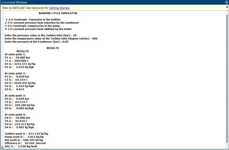
- Then the results were printed out for each four points and for the outputs.
Plots:
1.
2.
Result outout command window:
Reference: