Week 4.1 - Genetic Algorithm

Aim : To understand the concept of genetic algorithm and write a code in MATLAB to optimise the stalagmite function.

Genetic algorithm

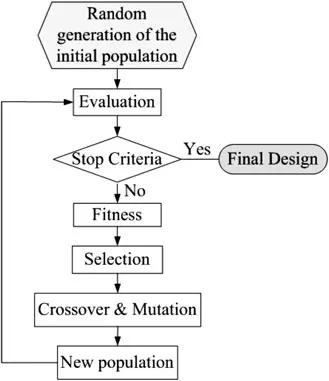
A genetic algorithm (GA) is a method for solving both constrained and unconstrained optimization problems based on a natural selection process that mimics biological evolution. The algorithm repeatedly modifies a population of individual solutions. At each step, the genetic algorithm randomly selects individuals from the current population and uses them as parents to produce the children for the next generation. Over successive generations, the population "evolves" toward an optimal solution.

You can apply the genetic algorithm to solve problems that are not well suited for standard optimization algorithms, including problems in which the objective function is discontinuous, nondifferentiable, stochastic, or highly nonlinear.

The genetic algorithm differs from a classical, derivative-based, optimization algorithm in two main ways, as summarized in the following table.

Classical Algorithm	Genetic Algorithm
Generates a single point at each iteration. The sequence of points approaches an optimal solution.	Generates a population of points at each iteration. The best point in the population approaches an optimal solution.
Selects the next point in the sequence by a deterministic computation.	Selects the next population by computation which uses random number generators.

Principal function of a simple genetic algorithm

Program for genetic algorithm:

In this below set of codes we will see how to use and the purpose of the function called 'ga'. For that we will see three kind of study which is 1.unbounded limits 2.bounded limits 3.limits with population size

First of all we have to creat the function program and named as 'stalagmite'.

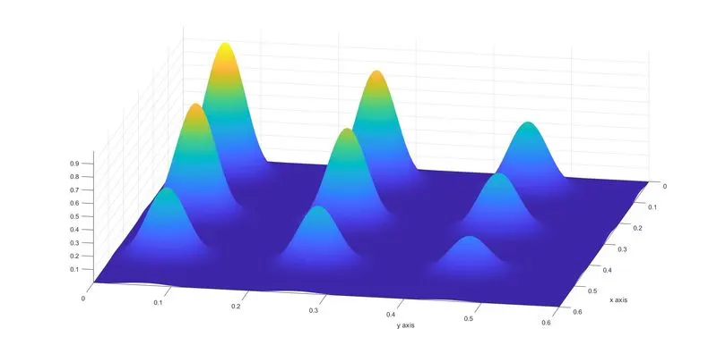
function f = stalagmite(input)
    x = input(1);
    y = input(2);
    f1_x = (sin((5.1*pi*x)+0.5)).^6;
     f2_x = exp(-4*log(2)*(((x-0.0667).^2)/0.64));
    f1_y = (sin((5.1*pi*y)+0.5)).^6;
    f2_y = exp(-4*log(2)*(((y-0.0667).^2)/0.64));
    f = -(f1_x*f2_x*f1_y*f2_y);
end     

After creating the function program the main program have to be written by using the function program.

clear all
close all
clc

%inputs
x= linspace(0,0.6,150);
y = linspace(0,0.6,150);
n=50;

%mesh
[xx,yy] = meshgrid(x, y);

%for loop for stalagmite
for i=1:length(xx)
    for j=1:length(yy)
        input_vector(1)=xx(i,j);
        input_vector(2)=yy(i,j);
        k(i,j)=stalagmite(input_vector);
    end
end    

%study 1 

tic
for j = 1:n
        [inputs,fval(j)] = ga(@stalagmite,2)
        input1(j) = inputs(1)
        input2(j) = inputs(2)
end
time=toc

figure(1)
subplot(2,1,1)
surfc(xx,yy,-k)
shading interp
hold on
plot3(input1,input2,-fval,'marker','o','markersize',5,'markerfacecolor','r')
xlabel('x axis');
ylabel('y axis');
subplot(2,1,2)
plot(-fval)
xlabel('iteration')
ylabel('function maximum')

%study 2
tic
for j = 1:n
        [inputs,fval(j)] = ga(@stalagmite,2,[],[],[],[],[0;0],[0.6;0.6])
        input1(j) = inputs(1)
        input2(j) = inputs(2)
end
time=toc

figure(2)
subplot(2,1,1)
surfc(xx,yy,-k)
shading interp
hold on
plot3(input1,input2,-fval,'marker','o','markersize',5,'markerfacecolor','r')
xlabel('x axis');
ylabel('y axis');
subplot(2,1,2)
plot(-fval)
xlabel('iteration')
ylabel('function maximum')

%study3
tic
for j = 1:n
        options=optimoptions('ga')
        options=optimoptions(options,'populationsize',250)
        [inputs,fval(j)] = ga(@stalagmite,2,[],[],[],[],[0;0],[0.6;0.6],[],[],options)
        input1(j) = inputs(1)
        input2(j) = inputs(2)
end
time=toc

figure(3)
subplot(2,1,1)
surfc(xx,yy,-k)
shading interp
hold on
plot3(input1,input2,-fval,'marker','o','markersize',5,'markerfacecolor','r')
xlabel('x axis');
ylabel('y axis');
subplot(2,1,2)
plot(-fval)
xlabel('iteration')
ylabel('function maximum')

In the above set of program we just saw the three type of cases like in

study no1, we simply execute the ga function by using stalagmite program without the boundry and also without the size of input. so, the output plots are given below

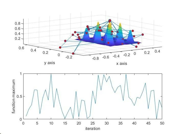
In the above plot we can see that the outpots are not in a proper condition. And also the matlab basically took the value 50 as the population size.

plots for study no.2

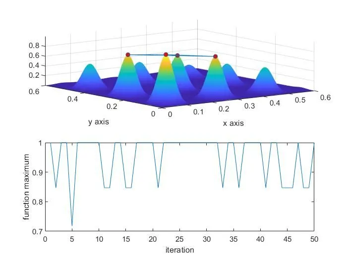
In second study we definded the boundry limits as 0 to 0.6. So, the result will be in our limits.

study 3 plots

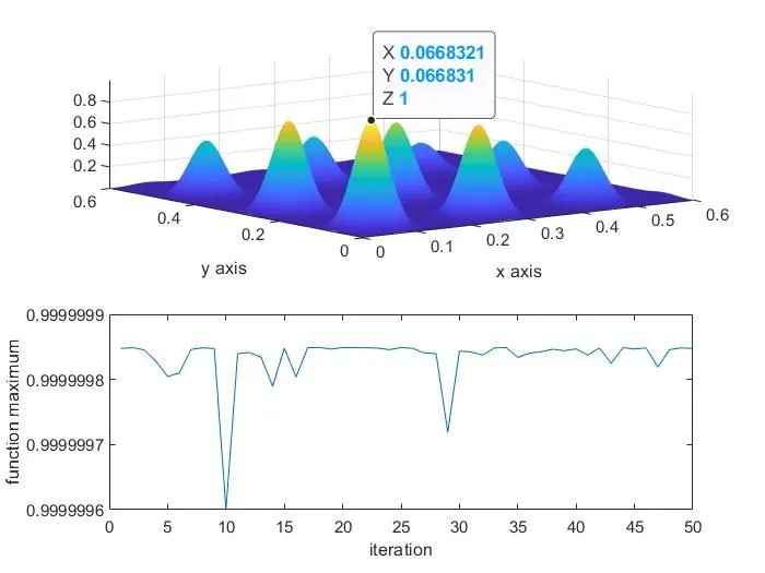
Here in case three we definded the boundry limit as well as the population size as 250. If we increase the no of population the result will be more linear.

References:

1.https://www.mathworks.com/discovery/genetic-algorithm.html

2.https://www.mathworks.com/help/gads/ga.html

3.https://en.wikipedia.org/wiki/Genetic_algorithm