Project 2

Project- Modeling a P1 Hybrid Electric Vehicle using matlab and simulink

Aim:

Development of a forward energy based fuel consumption model of a P1 hybird electric vehicle

Objectives:

This project deals with the development of a forward energy-based fuel consumption model of a P1 hybrid electric vehicle. The main goal is to understand the functionality of a P1 hybrid and be able to model it.

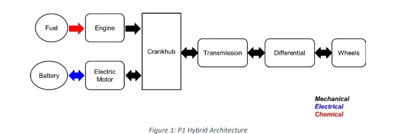
Honda Insight motor and battery are considered for this project. Data is taken from ADVISOR data base developed by NREL, USA.

Tasks:

The task of this project is to quantify the improvement in fuel economy numbers for the hybrid vehicle (kmpl), compared to the conventional vehicle, on the urban cycle (UDDS) and highway cycle (HWFET). Also, to analyze and understand the vehicle operating points in terms of engine and motor speed, torque, transmission speeds, pedal positions, gear, distance travelled, battery voltage, current, SoC etc. Make a report of the following observations

a. Tabulate the fuel economy numbers (kmpl) for UDDS and HWFET cycle. Compare these numbers with the baseline numbers for conventional vehicle model from Project 1.
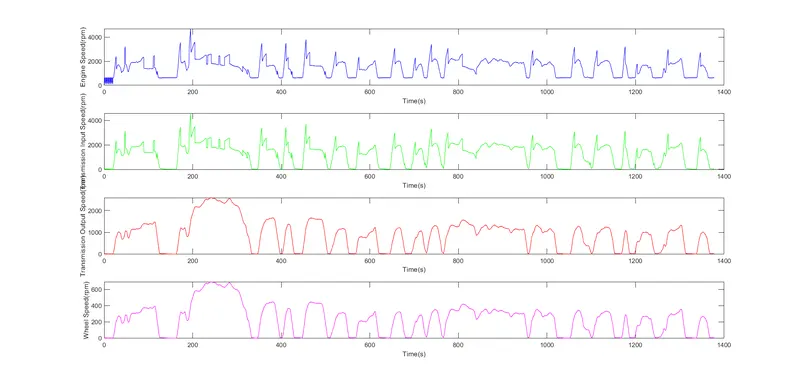
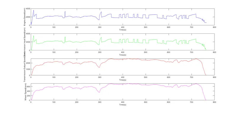
b. Plot the time trace for engine, transmission input, transmission output and wheel speed on one plot.
c. Plot engine torque, engine power, fuel rate and fuel consumption using subplots.
d. Plot accelerator and brake pedal, gear command, vehicle desired and actual speed, vehicle distance using subplots.
e. Plot the engine operating points on the engine fuel map.
f. Plot motor speed, torque, motor input power using subplots.
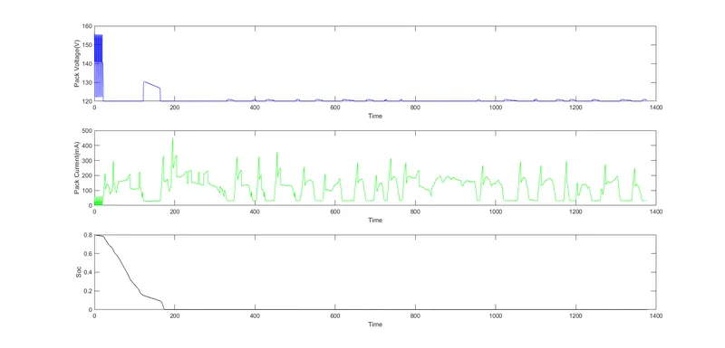
g. Plot pack voltage, current and SoC using subplots.
h. Plot the motor operating points on the motor input power map, with the motor max motoring and generating torque curves.
i. Write down appropriate brief comments on each of these plots, describing the vehicle behavior throughout the drive cycle.
j. Generate the plots for both drive cycles

Introduction:

For the given project, we have a P1 hybrid electric vehicle under consideration. Let’s dive deeper into the architecture of this type of parallel HEV. By architecture, topology or configuration we understand the positioning of the main components of the hybrid electric system on the vehicle. Since the only mechanical link between the electrical system and the rest of the vehicle is done through the electric machine, the HEV architecture is basically defined by the position of the electric machine and the type of connection with the powertrain / drivetrain (belt, integrated or gear mesh).

The powertrain configuration of the HEV system has significant impact on the performance and characteristics of the vehicle, in terms of:

• integration cost
• fuel efficiency
• dynamic performance (powertrain torque enhancement)

The electric machine can be positioned, relative to the other powertrain components, at five major points:

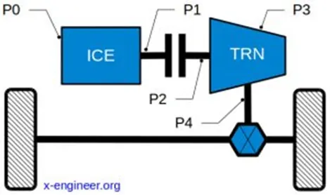
The brif description of the electric machine connections points is done in the below

• P0 The electric machine is connected with the internal combustion engine through a belt, on the front end accessory drive (FEAD)
• P1 The electric machine is connected directly with the crankshaft of the internal combustion engine
• P2 The electric machine is side-attached (through a belt) or integrated between the internal combustion engine and the transmission; the electric machine is decoupled from the ICE and it has the same speed of the ICE (or multiple of it)
• P3 The electric machine is connected through a gear mesh with the transmission; the electric machine is decoupled from the ICE and it’s speed is a multiple of the wheel speed
• P4 The electric machine is connected through a gear mesh on the rear axle of the vehicle; the electric machine is decoupled form the ICE and it is located in the rear axle drive or in the wheels hub

The P0 and P1 architectures do not allow the mechanical disconnection of the electric machine from the engine. On the other side P2, P3 or P4 configurations disconnects the electric machine from the engine through a clutch. In the P1 architecture, the electric machine is connected directly to the crankshaft. The electric motor functions as a generator, during vehicle deceleration, as an engine starter, and as a motor (to assist the engine) during vehicle accelerations.

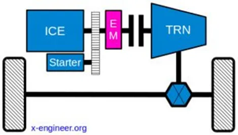
One of the biggest advantage of this solution is that the electric motor can provide higher torque, since there is no belt limitation (due to slip). However, since there is no speed / torque ratio between the electric machine and crankshaft, the torque requirements on the electric motor can be quite demanding. The main disadvantages of this type of architecture are it’s higher cost and higher impact on the existing vehicle architecture.

Two examples of P1 MHEV architectures are:

1. Honda Insight Hybrid 2009 (with Integrated Motor Assist technology)
2. Mercedes Benz S400 Bluehybrid 2010

Building the Model:

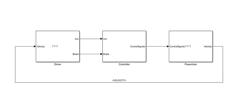
Based on the vehicle architecture discussed above, we shall build a Simulink model representing the system. For it, lets consider the system to be an integration of three interfaces:

- Surrounding-Driver interface

- Driver-Controller interface

- Controller-Powertrain interface

The vehicle behaviour is an outcome of the interdependent functioning of these interfaces. We shall build our model in a way, such that, each interface is a separate subsystem with its outputs and inputs linked to the other two in some way or the other.

Driver:

The driver is the initiator of each and every movement of the vehicle. All the reactions of the vehicle are a response to the driver inputs, directly or indirectly. The driver assesses the surrounding conditions and based on his intellectual instincts, provides corresponding inputs to the vehicle. The inputs are basically mechanical motions which are converted to digital signals by the controller. Driver subsystem can thus be modelled as:

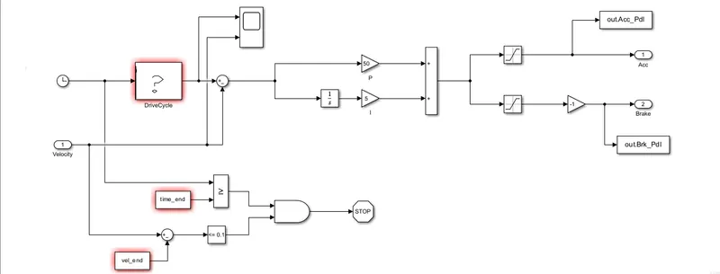
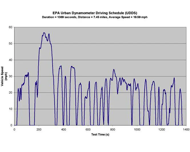
Here, the surroundings are taken as approximations of typical driving conditions in common occurrence. These are built in the form of Drive cycles, which are ‘Velocity vs Time’ charts based on certain driving conditions. The desired speed from the drive cycle is compared against the actual speed output of the vehicle. The difference of the two is the error and this error is provided with the proportional and integral gains for the feedback control of the system. The speed is capped at 100 using the saturation blocks, both for the forward and rearward motions of the vehicle, for our case. Based on what action is necessary, the driver presses on the accelerator or brake pedals to control the vehicle. These are the inputs to the controller subsystem. Also, at the end of the drive cycle the engine needs to stop and the same has been provisioned.

Controller:

The controller unit is the brain of the vehicle. It firstly converts inputs received from the Driver into digital signals. Based on these signals, it generates outputs to be sent to the various powertrain components based on a set of algorithms. Controller unit can thus be modelled as:

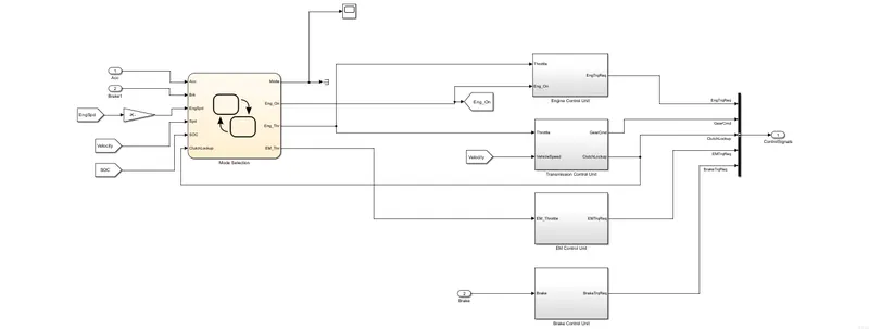
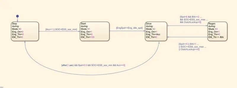
Based on the driver inputs and feedbacks from the vehicle components, the controller needs to make decisions on the mode it needs to select, for the vehicle to operate in. This is done using a Stateflow chart. The inputs to the chart are the acceleration pedal input, the brake pedal input, instantaneous engine speed, instantaneous vehicle velocity, SoC (state of charge) of the battery and the clutch lockup status. Based on these inputs, the model selector decides which mode the vehicle is to be operated in from: conventional, electric, hybrid or regenerative braking. The outputs from the selector are then sent to the component controllers. For our case they are 4 in number:

Engine Control Unit

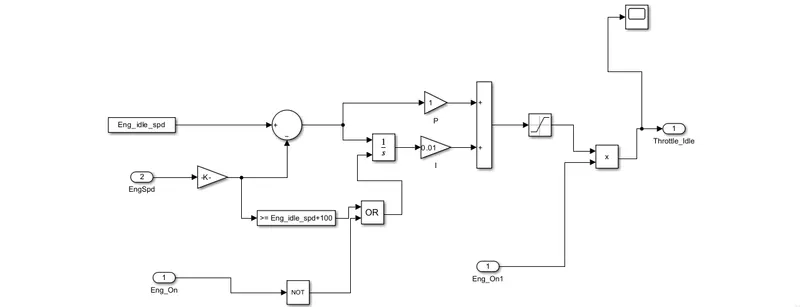
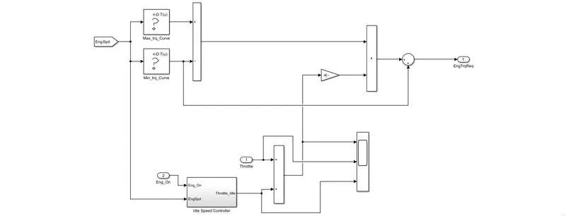
The inputs to this unit are throttle and engine on/off inputs. As this is a hybrid vehicle, the engine can be shut off during idling or low power applications. In the subsystem, based on the engine speed and the throttle input, the controller decides what torque is required to be generated by the engine to meet the vehicle demands. This is done based on torque and speed maps using ‘lookup tables’ that interpolate the values based on these inputs. This subsystem can thus be modelled as:

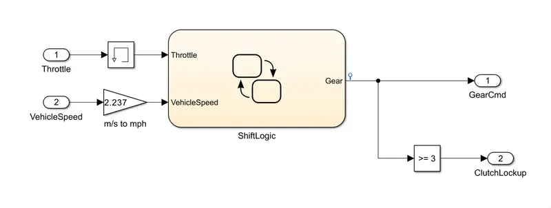
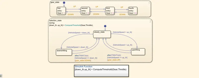
Transmission Control Unit

The inputs to this subsystem are the throttle and vehicle speed. Based on these inputs, the shift logic decides the gear ratio that the vehicle needs to operate in for optimum efficiency. Also, as the vehicle under consideration has a torque converter unit, the clutch lockup is also decided. The condition for it here is given as, for gears higher than or equal to the third gear, the turbine will be locked to the engine output for direct transmission. This subsystem can thus be modelled as:

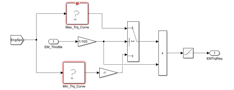
Electric Machine Control Unit

The input to this subsystem is the throttle for the electric machine, which is nothing but the current control. As the electric machine in a P1 hybrid is mounted directly on the engine crankshaft, the input speed for the motor is the engine speed. Based on the throttle input the controller decides the torque to be generated by the motor (based on torque and speed maps). This subsystem can thus be modelled as:

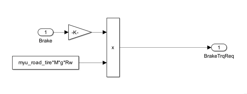
Brake Control Unit

The input to this subsystem is the brake pedal input from the driver. Based on this input and the Rolling resistance force, the controller decides the amount of brake torque required to meet the braking demands. The subsystem can thus be modelled as:

There are 5 outputs from the subsystem and they are transmitted via the bus creator

Powertrain

The powertrain unit of the vehicle is where the power to move the vehicle is generated, conditioned to upscale or downscale and transmitted to the wheels. It thus consists of the engine/motor (energy converters), gearbox/torque converter (energy transformers), Differential (energy splitters) and wheels (energy consumers). Each of these are modelled as separate subsystems.

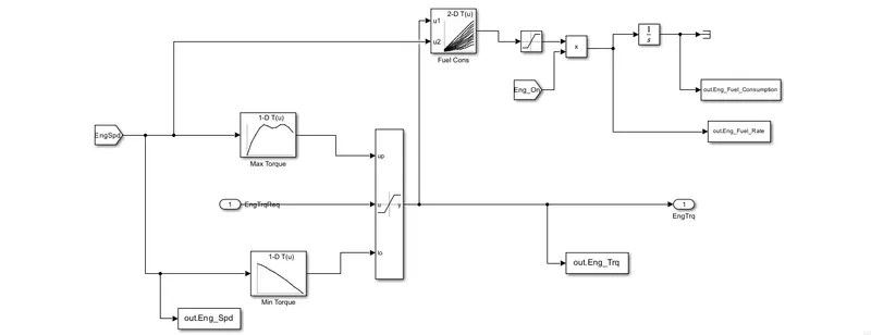
Engine

For the P1 type of HEV, engine is the primary energy converter. The required torque output signal developed by the controller acts as an input for this subsystem. Based on this input and the engine speed, the engine develops corresponding torque. The output torque however is bounded by the maximum/minimum torque that can be generated corresponding to the engine speed. Also, the fuel consumption rate is calculated based on the engine fuel maps. The engine can thus be modelled as:

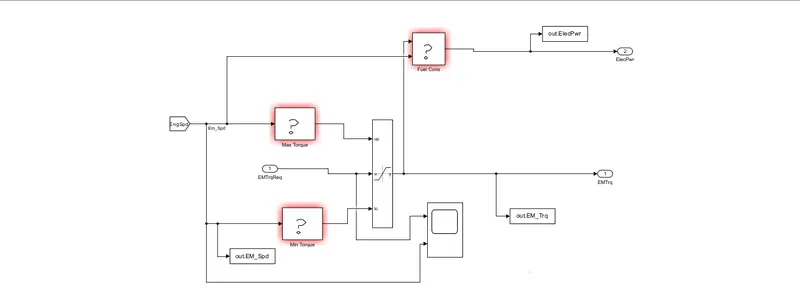
Electric Machine

As discussed above, the electric machine in a P1 hybrid is mounted on the engine crankshaft just after the engine. Again here the torque required to be generated by the motor, whenever the vehicle is operated in hybrid or electric mode, is calculated by the controller. This acts as an input to the motor. Based on the speed of the motor, which is the speed of the engine itself, the motor generates the required torque. In addition, the power that the motor requires to draw from the battery pack is estimated and sent to the battery pack. The electric machine subsystem can thus be modelled as:

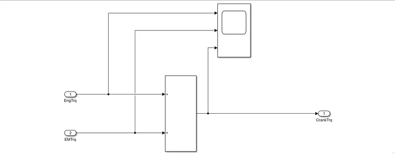
Crank Hub

While operating in the hybrid mode, the output at the crankshaft would be the addition of the outputs from the engine and the electric machine. This subsystem adds the outputs of the two and feeds it to the transmission. This subsystem can be modelled as:

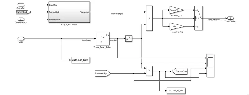
Transmission

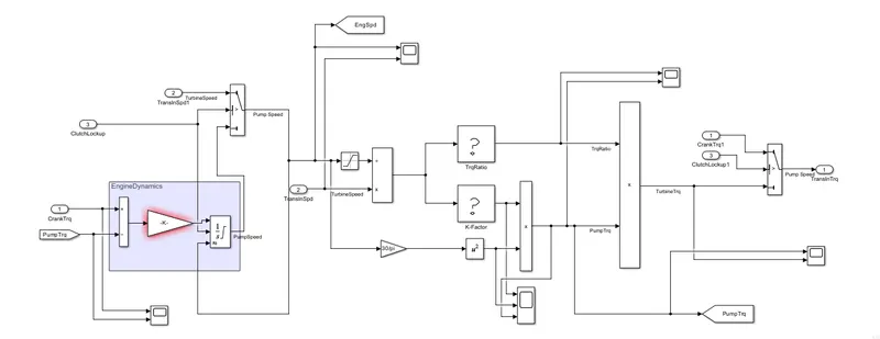
The transmission comprises of the torque converter and the transmission shafts. In the torque converter, the torque coming from the crankshaft is scaled up or down based on the requirements at the wheels. Say in case the vehicle is moving uphill, the torque demanded by the vehicle in such instances is high. Hence, the torque converter needs to scale up the crank torque. The torque converter is a separate subsystem in transmission. The inputs to it are the crank torque, transmission input speed and the clutch lockup status. The difference between the new generated crank torque and the previous pump torque is the error that the torque converter needs to correct. When divided by the inertias of the engine and motor, the pump speed is obtained. Then based on the clutch lockup status the turbine speed is decided. Using the torque ratio and K-factor maps, the turbine torque is estimated and acts as the input torque to the transmission shaft. Then based on the selected gear and the efficiency of the transmission the output torque is estimated. The transmission subsystem can thus be modelled as:

Differential

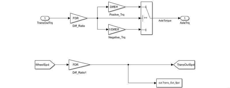
The differential does the function of torque distribution between the driving wheels based on the drive ratio. The differential efficiency as well comes into play here. The differential can be modelled as:

Wheels

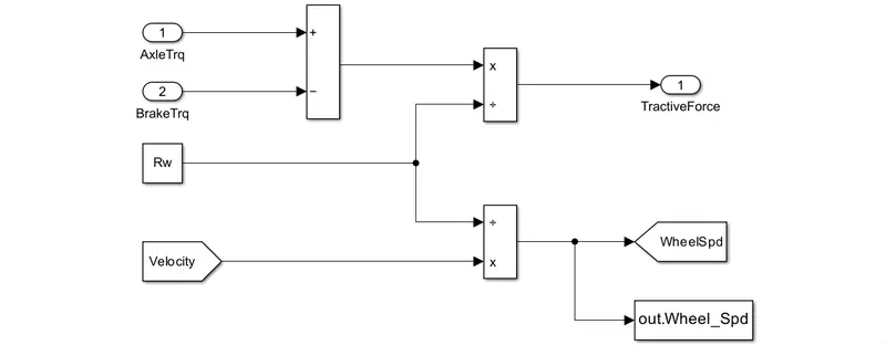
The torque after being transmitted through the transmission is provided to the wheels. Also, the brake torque is taken as an input here as the brake is applied directly to the wheels. The rolling resistance of the wheel is a factor of consideration as well. The wheel can be modelled as:

Battery Pack

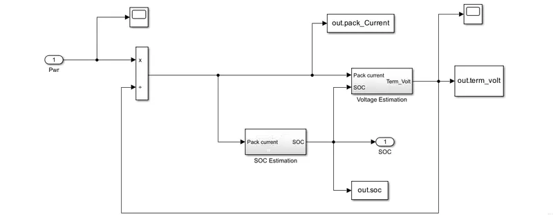
The battery pack is the fuel storage unit of the motor. Based on the power demanded by the motor, the battery pack has to provide it instantaneously and also store the energy during regenerative braking. The battery pack also has to maintain its state of charge in HEVs other than the plug-in HEVs.

Vehicle Dynamics

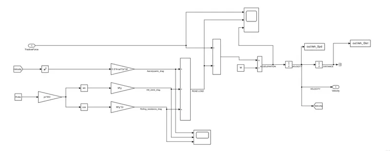
This block is nothing but the estimation of the vehicle velocity after overcoming the drag due to aerodynamics of the vehicle, drag due to rolling resistance of the wheels and the drag due to ascending or descending a gradient. The block is thus implemented as:

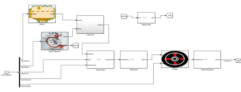
AS a whole, the powertrain subsystem can be configured as :

The vehicle model based on these subsystems can thus be configured as:

Initialization script:

%% Initialization File
% Initialization file for loading the variables for the Conventional vehicle simulation model

%% Vehicle Parameters
M = 1500;       % Vehicle weight [kg]
Cr = 0.015;     % Rolling resistance coefficient
Rw = 0.35;      % Rolling radius [m]
Cd = 0.33;      % Drag coefficient
Af = 2;         % Frontal area [m2]
rhoa = 1.225;   % Air density [kg/m3]
Vwind = 0;      % Wind velocity [kmph]
g = 9.81;       % Gravitational acceleration [m/s2]
theta = 0;      % Slope [deg]
myu_road_tire = 1; % Coefficient of friction between tire - road interface

%% Powertrain Parameters 
FDR = 3.73;                         % Final Drive Ratio / Diff Ratio
DiffEff = 0.99;                     % Differential efficiency (assumed independent of operating conditions)

NumGear = 4;                        % Number of gears in transmission
TransGear = [1:NumGear];            % Transmission Gears
TransRatio = [3.06, 1.62, 1, 0.7];  % Corresponding Transmission ratios
TransEff = 0.90;                    % Transmission efficiency (assumed independent of operating conditions)

TC_SR = [0, .5, .6, .7, .8, .87, .92, .94, .96, .97, 1];   % Torque Converter Speed Ratio (Matlab default) -> TurbSpd/PumpSpd  
TC_TR = [2.232, 1.5462, 1.4058, 1.2746, 1.1528, 1.0732, 1.0192, 1, 1, 1, 1];   % Torque Converter Torque Ratio (Matlab default) -> TurbTrq/PumpTrq
TC_Cf = 1e-4 * [.72558, .66322, .63463, .59042, .51331, .4144, .29287, .22444, .12186, .04386, 0]; % Torque Converter Capacity Factor (Matlab default) -> PumpTrq/PumpSpd^2 [Nm/rpm^2]

load Vehicle_Data/Engine_data_1_9L_Saturn_95kW
load Vehicle_Data/Trans_Shift_map
load Vehicle_Data/EM_Honda_Insight_10kW
load Vehicle_Data/ESS_NiMH6


ESS_init_soc = 0.8;
ESS_soc_max = 0.9;
ESS_soc_min = 0.6;


%% Driver Parameters
Kp = 10;                    % P gain for driver PI model
Ki = 1;                     % I gain for driver PI model
Drive_Cycle_Select = 1;     % Drive cycle selection

% Drive cycle values in m/s

if Drive_Cycle_Select == 1
    load DriveCycles/UDDS;
    
elseif Drive_Cycle_Select == 2
    load DriveCycles/HWFET;
    
elseif Drive_Cycle_Select == 3
    load DriveCycles/FTP;
    
elseif Drive_Cycle_Select == 4
    load DriveCycles/US06;
    
elseif Drive_Cycle_Select == 5
    load DriveCycles/NEDC;
    
elseif Drive_Cycle_Select == 6
    load DriveCycles/WLTP;
 
end

time_end = cyc_time(end);
vel_end = cyc_vel(end);

Post Processing script

For generating the output plots as well a script can be coded. It is based on the variables sent to the workspace. The code for it is:

%% Post-Processing File
 %File for post-processing the Conventional vehicle simulation model data

%% Renaming variables
Time = out.tout;
Acc_Pdl = out.Acc_Pdl;          % Accelerator pedal [%]
Brk_Pdl = out.Brk_Pdl;          % Brake pedal [%]
Gear_Cmd = out.Gear_Cmd;        % Transmission gear
Trans_In_Spd = out.Trans_In_Spd*30/pi;  % Transmission input speed [rpm]
Trans_Out_Spd = out.Trans_Out_Spd*30/pi;% Transmission output speed [rpm]
Eng_Trq = out.Eng_Trq;          % Engine brake torque [Nm]
Eng_Spd = out.Eng_Spd*30/pi;% Engine speed [rpm]
Eng_Fuel_Rate = out.Eng_Fuel_Rate; %Engine Fuel Consumption rate
Eng_Fuel_Consump = out.Eng_Fuel_Consumption;    % Engine fuel consumption [g]
Veh_Dist = out.Veh_Dist/1000;   % Distance traveled by vehicle [km]
Veh_Spd = out.Veh_Spd*18/5;     % Vehicle speed [kmph]
Wheel_Spd = out.Wheel_Spd*30/pi; % Wheel speed [rpm]
EM_Trq = out.EM_Trq; % Motor Torque [Nm]
EM_Spd = out.EM_Spd; %Motor Speed [rpm]
EM_In_Pwr = out.ElecPwr; %Motor Input Power[kW]
Pack_voltage = out.term_volt; %Pack Voltage[V]
Pack_current = out.pack_Current; %Pack Current[A]
SoC = out.soc; %State of Charge
%% Data Analysis
Eng_Pwr = Eng_Spd*pi/30.*Eng_Trq/1000;   % Engine brake power [kW]
rho_petrol = 0.7197;                    % Density of petrol [kg/L]
kmpl = Veh_Dist(end)/(Eng_Fuel_Consump(end)/1000/rho_petrol);    % Fuel economy [kmpl] 


%% Plotting vehicle characteristics time trace
figure('Name','Time Trace')
subplot(411);plot(Time,Eng_Spd,'b-');xlabel('Time(s)');ylabel('Engine Speed(rpm)')
subplot(412);plot(Time,Trans_In_Spd,'g-');xlabel('Time(s)');ylabel('Transmission Input Speed(rpm)')
subplot(413);plot(Time,Trans_Out_Spd,'r-');xlabel('Time(s)');ylabel('Transmission Output Speed(rpm)')
subplot(414);plot(Time,Wheel_Spd,'m-');xlabel('Time(s)');ylabel('Wheel Speed(rpm)')
%% Plotting engine operating points on engine fuel map
figure('Name','Engine Operating Points');
hold on
grid on
title('Engine Operating Points','fontsize',12);
p1=plot(Eng_map_spd*30/pi,Eng_max_trq,'linewidth',2,'color','r');
p2=line([Eng_map_spd(end)*30/pi Eng_map_spd(end)*30/pi],[0 Eng_max_trq(end)]);
set(p2,'linewidth',1,'linestyle','--','color','k');
p3=line([Eng_map_spd(1)*30/pi Eng_map_spd(1)*30/pi],[0 Eng_max_trq(1)]);
set(p3,'linewidth',1,'linestyle','--','color','k');
[c,h] = contour(Eng_map_spd'*30/pi,Eng_map_trq,Eng_fuel_map');
clabel(c,h);
xlabel('Engine Speed [rpm]');
ylabel('Engine Torque [Nm]');
title('Engine Fuel Consumption Map [g/s]');
p4 = plot(Eng_Spd,Eng_Trq,'.','color','k');
legend([p1 p4],{'Max Torque Curve','Operating Points'});
axis([Eng_map_spd(1)*30/pi Eng_map_spd(end)*30/pi 0 Eng_map_trq(end)]);

%% Plotting Engine performance parameters
figure('Name','Engine Performance Parameters')
subplot(411);plot(Time,Eng_Trq,'b-');xlabel('Time');ylabel('Engine Torque')
subplot(412);plot(Time,Eng_Pwr,'g-');xlabel('Time');ylabel('Engine Power')
subplot(413);plot(Time,Eng_Fuel_Rate,'k-');xlabel('Time');ylabel('Engine Fuel consumption rate')
subplot(414);plot(Time,Eng_Fuel_Consump,'m-');xlabel('Time');ylabel('Engine Fuel Consumption')

%% Plotting Vehicle Parameters
figure('Name','Vehicle parameters')
subplot(321);plot(Time, Acc_Pdl, 'b-');title('Acceleration Pedal');
xlabel('Time(s)');ylabel('Pedal[%]')
subplot(322);plot(Time, Brk_Pdl, 'g-');title('Brake Pedal');
xlabel('Time(s)');ylabel('Pedal[%]')
subplot(323);plot(Time, Gear_Cmd, 'r-');title('Gear command');
xlabel('Time(s)');ylabel('Gear engaged')
subplot(324);plot(cyc_time,2*cyc_vel*1.609,'b-');title('Desired Vehicle Speed');
xlabel('Time(s)');ylabel('Speed(kmph)')
subplot(325);plot(Time,Veh_Dist,'c-');title('Distance travelled by Vehicle')
xlabel('Time(s)');ylabel('Distance(km)')
subplot(326);plot(Time,Veh_Spd,'m-');title('Actual Vehicle Speed');
xlabel('Time(s)');ylabel('Speed(kmph)')

%%
% Motor parameters
figure('Name','Motor Performance Parameters')
subplot(311);plot(Time,EM_Spd,'b-');xlabel('Time');ylabel('Motor Speed(rpm)')
subplot(312);plot(Time,EM_Trq,'g-');xlabel('Time');ylabel('Motor Torque(Nm)')
subplot(313);plot(Time,EM_In_Pwr,'k-');xlabel('Time');ylabel('Motor Input Power(W)')

%%
figure('Name','Battery Performance Parameters')
subplot(311);plot(Time,Pack_voltage,'b-');xlabel('Time');ylabel('Pack Voltage(V)')
subplot(312);plot(Time,Pack_current,'g-');xlabel('Time');ylabel('Pack Current(mA)')
subplot(313);plot(Time,SoC,'k-');xlabel('Time');ylabel('Soc')

%% Plotting engine operating points on engine fuel map
figure('Name','Motor Operating Points');
hold on
grid on
title('Motor Operating Points','fontsize',12);
p1=plot(EM_map_spd*30/pi,EM_max_trq,'linewidth',2,'color','r');
p2=line([EM_map_spd(end)*30/pi EM_map_spd(end)*30/pi],[0 EM_max_trq(end)]);
set(p2,'linewidth',1,'linestyle','--','color','k');
p3=line([EM_map_spd(1)*30/pi EM_map_spd(1)*30/pi],[0 EM_max_trq(1)]);
set(p3,'linewidth',1,'linestyle','--','color','k');
[c,h] = contour(EM_map_spd'*30/pi,EM_map_trq,EM_inpwr_map');
clabel(c,h);
xlabel('Motor Speed [rpm]');
ylabel('Motor Torque [Nm]');
title('Motor Fuel Consumption Map [g/s]');
p4 = plot(EM_Spd,EM_Trq,'.','color','k');
legend([p1 p4],{'Max Torque Curve','Operating Points'});
axis([EM_map_spd(1)*30/pi EM_map

Outputs:

1.UDDS(Urban dynamometer driving schedule) cycle:

a.Mileage(in kmpl)

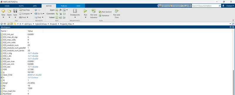
The mileage (in kmpl) for the P1 hybrid under consideration is obtained as 25.38 kmpl, whereas, for a conventional vehicle it is obtained as 20.29 kmpl. This shows that with the addition of a secondary power source the efficiency of the engine improves

b.Time trace

c. Engine parameters

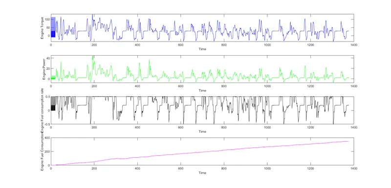
As the drive cycle is based on urban driving conditions, there are frequent start and stops in the cycle and hence the fluctuating nature of the first three graphs. The vehicle consumes around 215 grams of fuel for the journey.

d. Vehicle parameters

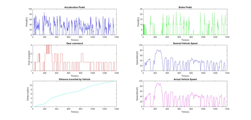
As can be seen, the desired vehicle speed plot and the actual vehicle speed plots are in close resemblance to each other. This goes on to prove that our model is able to perform the required tasks demanded off the system. The vehicle operates in lower gears for most part of the cycle and travels about 12 kms. There's frequent engagement of the brake pedal as well.

e. Engine operation points

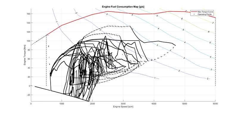
The engine operates in the lower to middle section of the plot. Though it is not the highest efficiency of the engine, there is an increase as compared to the conventional vehicle. It is so because at lower speeds and torques the electric machine comes into play and hence reduces the idling losses.

f. Electric machine parameters

The electric machine here does the work of providing the starting torques for the vehicle. Also, during braking it facilitates regenerative braking.

h. Electrc machine operating points

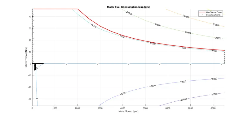
The electric machine operates both in the forward and the reverse modes, as a motor and a generator respectively.

2.HWFET(Highway fuel economy test) cycle:

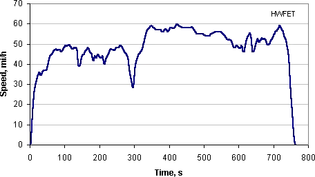
a.Mileage (in kmpl)

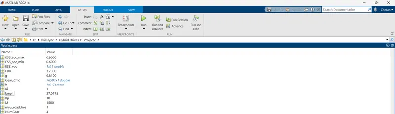
The mileage for the hybrid cycle is 37.02 kmpl, whereas for a conventional vehicle, for the same drive cycle, the mileage is obtained as 29.11 kmpl. Again it validates the improvement in efficiency of the engine with addition of a secondary source of power.

b. Time trace

c. Engine parameters

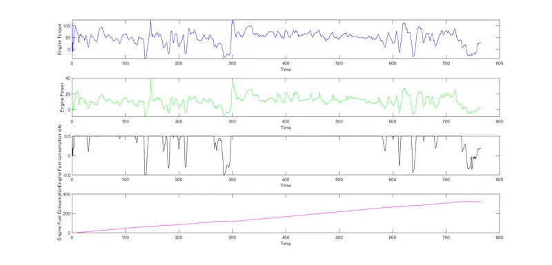
As the HWFET cycle is representative of Highway driving conditions, there are lesser fluctuations in the torque and power graphs. The engine consumes about 302 grams of fuel during the journey.

d. Vehicle parameters

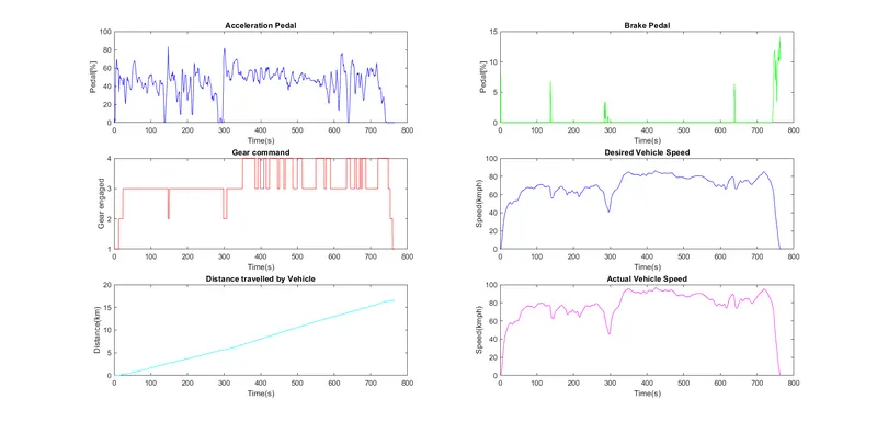
The vehicle here operates in the higher gears for most parts of the journey. There's reduced use of the brake pedal as compared to the UDDS cycle. The vehicle travels about 16 kms in a relatively shorter period of time.

e. Engine operating points

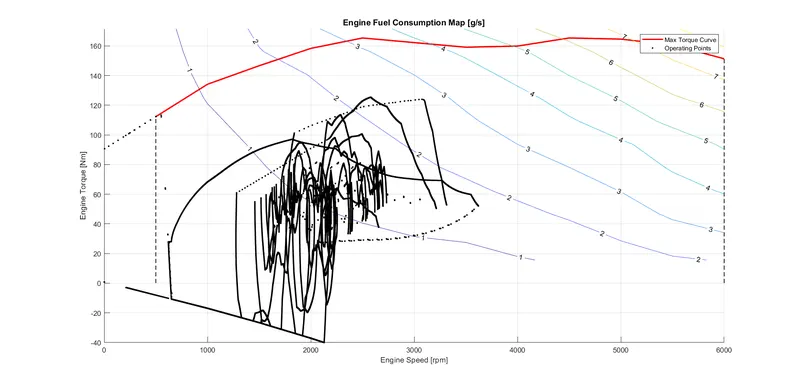
For this cycle, the engine operates mostly near the middle region of the graph which is the better efficiency region.

f. Electric machine parameters

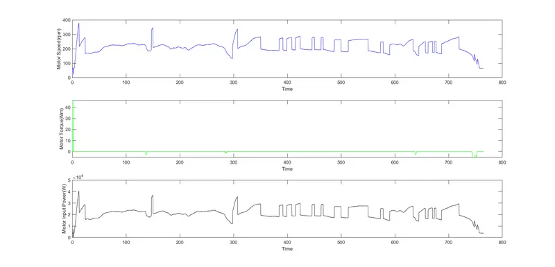
For this cycle, there isn't much scope to operate the motor other than starting the enigne and providing the initial torque. Also, as there isn't much braking, regenerative braking doesn't come into play much.

g. Battery parameters

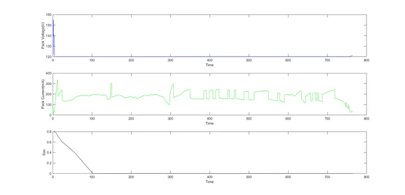
h. Electric machine operating points

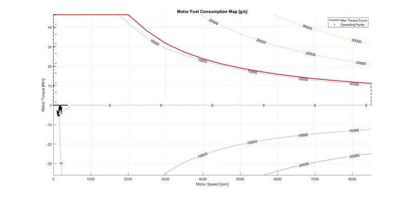
The EM operating points for both the cycles are nearly the same as the battery pack in use is of a lesser capacity and hence exhausts early.

Conclusion:

In this project, we got to know about the architecture of a P1 Hybrid Electric Vehicle (HEV) and how to model it using MATLAB & Simulink. We obtained various performance parameters for the vehicle based on different drive cycles and compared those against the parameters of a conventional vehicle. In comparison we found the HEV to have improved performance parameters as against the conventional vehicle, due to the addition of a secondary power source.