Project 2
Project-2
Question:
As discussed in Lecture 11, Project 2 deals with the development of a forward energy-based fuel consumption model of a P1 hybrid vehicle. This model is based on the conventional vehicle model from Project 1.
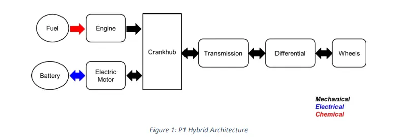
The main goal of this project is to understand the functionality of a P1 hybrid and be able to model it.
Honda Insight motor and battery are considered for this project. Data is taken from the ADVISOR database developed by NREL, USA. Data is provided in the project files.

“Project2_InitFile.m” is a Matlab script used to load all the variables required for running the Simulink model and for post-processing. The drive cycle selection is also done here. Before running the Simulink vehicle model, run this initialization script.
Task:
The task of this project is to quantify the improvement in fuel economy numbers for the hybrid vehicle (kmpl), compared to the conventional vehicle, on the urban cycle (UDDS) and highway cycle (HWFET). Also, to analyze and understand the vehicle operating points in terms of engine and motor speed, torque, transmission speeds, pedal positions, gear, distance traveled, battery voltage, current, SoC, etc.
To do that, the following steps need to be followed:
1) Load the Project2 folder as the Current Folder in Matlab.
2) Run the “Project2_InitFile.m” Matlab script.
3) Copy the Conventional vehicle Simulink model created for Project 1 in this folder. Figure 1: P1 Hybrid ArchitectureHybrid Drives Development
4) Modify this model into a hybrid vehicle model. The lecture presentations can be used as a reference. Battery and Supervisory controller models developed in the assignments can be reused.
5) Add additional ‘To Workspace’ blocks for transferring the desired Simulink vehicle data into the Matlab workspace.
6) Simulate the hybrid model on the desired drive cycles.
7) Write a project report that contains the following:
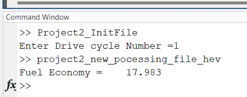
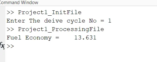
a. Tabulate the fuel economy numbers (kmpl) for UDDS and HWFET cycle. Compare these numbers with the baseline numbers for conventional vehicle model from Project 1.
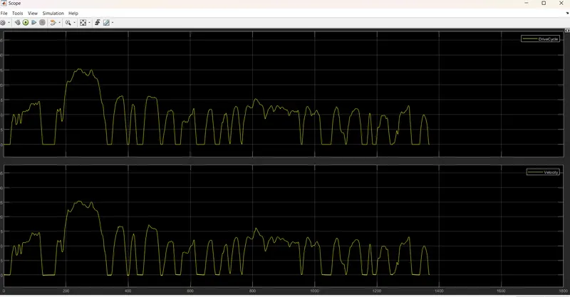
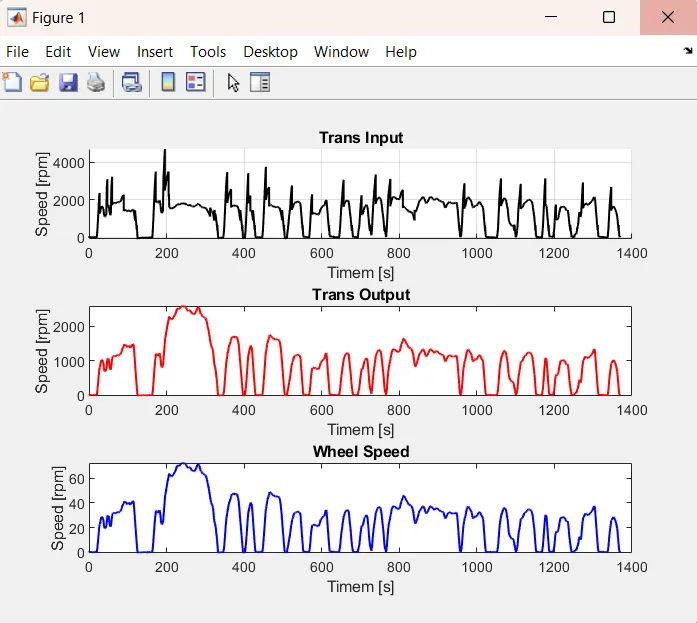
b. Plot the time trace for engine, transmission input, transmission output and wheel speed on one plot.
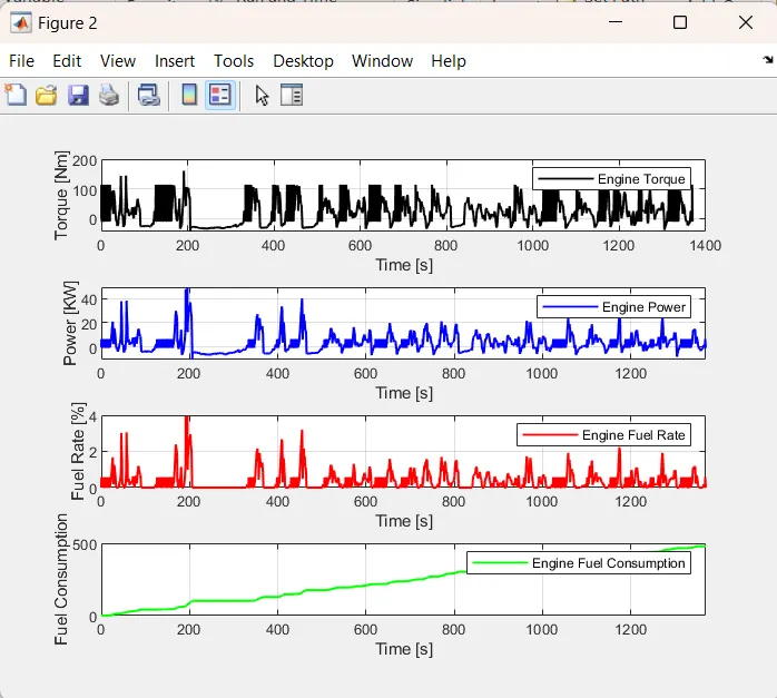
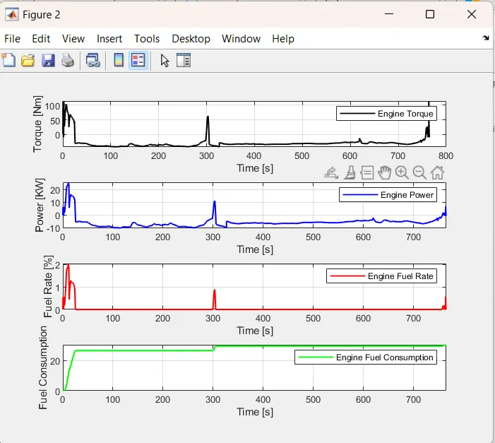
c. Plot engine torque, engine power, fuel rate and fuel consumption using subplots.
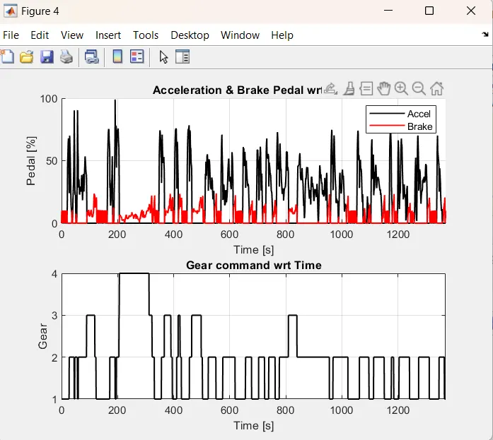
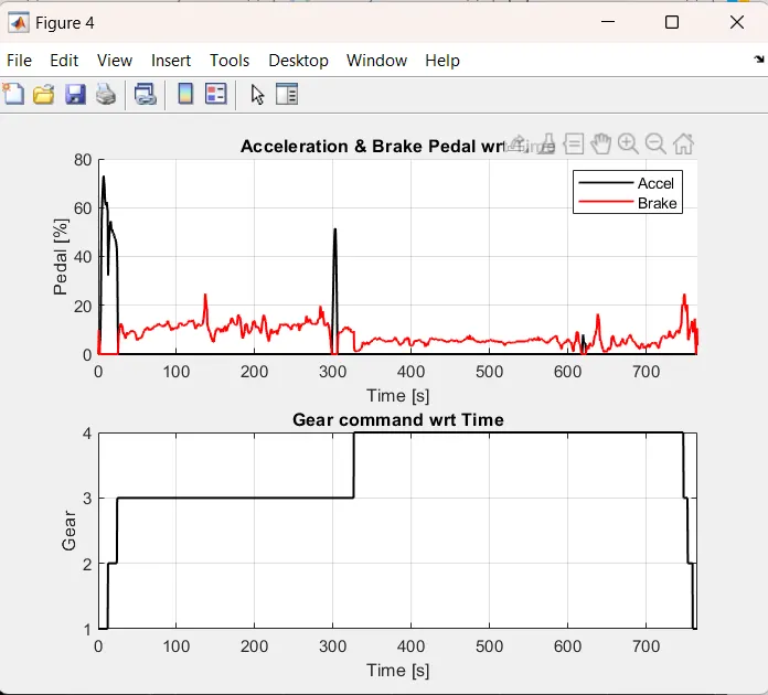
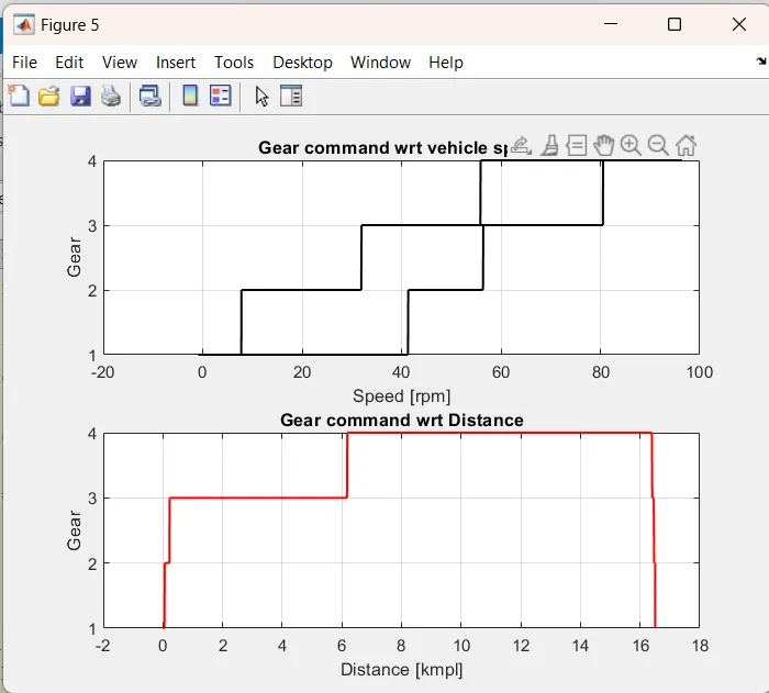
d. Plot accelerator and brake pedal, gear command, vehicle desired and actual speed, vehicle distance using subplots.
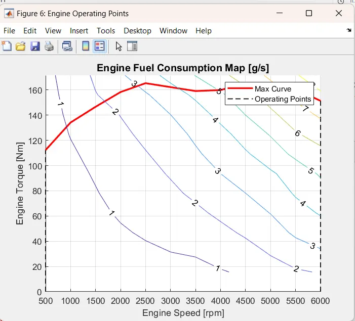
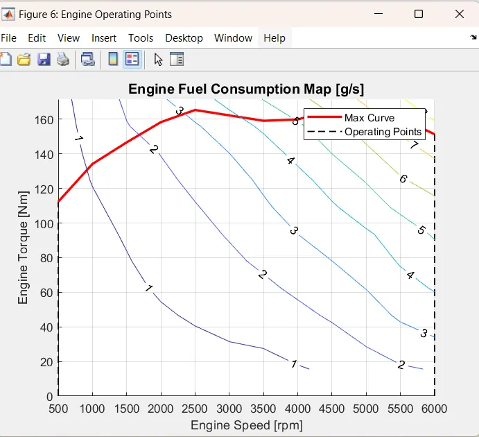
e. Plot the engine operating points on the engine fuel map.
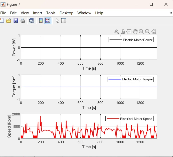
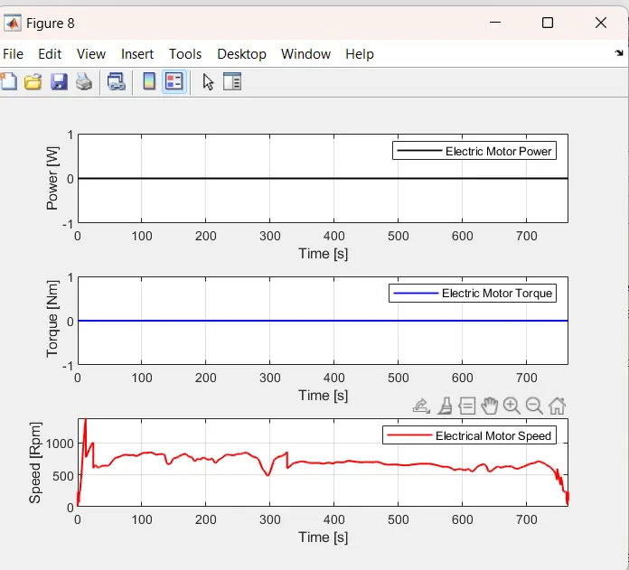
f. Plot motor speed, torque, motor input power using subplots.
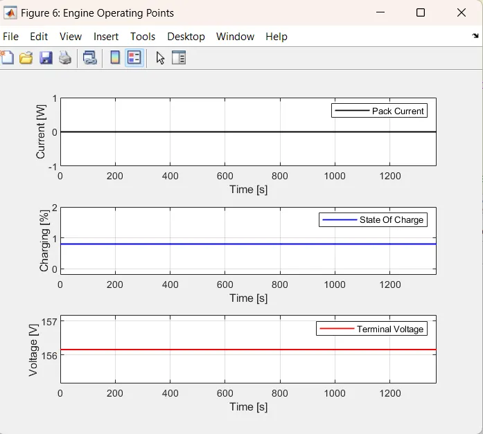
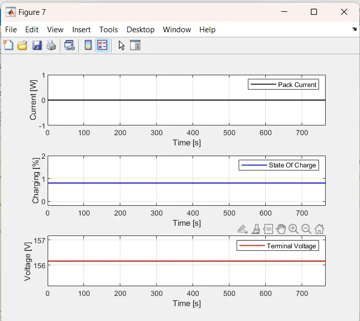
g. Plot pack voltage, current and SoC using subplots.
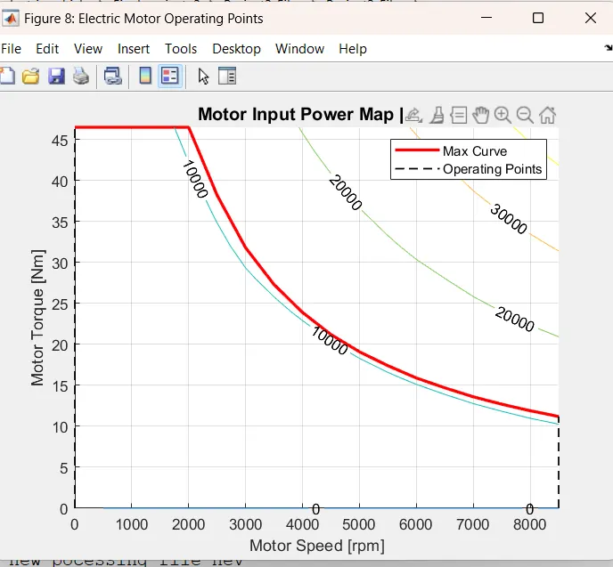
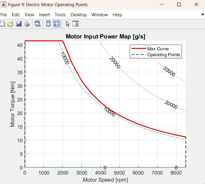
h. Plot the motor operating points on the motor input power map, with the motor max motoring and generating torque curves.
i. Write down appropriate brief comments on each of these plots, describing the vehicle behavior throughout the drive cycle.
j. Generate the plots for both drive cycles
Project 2- Development of a forward energy-based fuel consumption model of a P1 hybrid vehicle.
Forward Models.
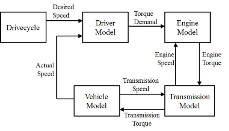
Forward models are utilized for detailed simulations, whereas dynamic models are used for forwarding models (refer to Figure 1). The input is force/torque/power, and the outputs are the vehicle state variables velocity and acceleration. Because physical casualty makes models and simulations more realistic, they are better for control development. To achieve the desired vehicle state, there is a feedback loop. Because of the dynamics, the simulation is slower, and the approach is mostly used to model a vehicle drive cycle and study the system's dynamic behaviour. Significantly aids in the management of development.

A forward-facing vehicle model features a driver model that provides torque demand in the form of desired ICE torque and brake torque, to meet the speed trace from a drive cycle. The topology of the forward-facing model that is used in this investigation is shown in Figure 1. A basic driver model typically uses one or more Proportional-Integral (PI) controllers to achieve the torque demand, concerning the desired speed trace. This is discussed further in the next section. The torque produced by the ICE propagates through the transmission and final drive ratios, before ending up as torque applied at the wheels. This is then exerted on the vehicle mass via force on the tire contact patch. The vehicle speed that results from the applied force is propagated back through the drivetrain and returns to the ICE as angular velocity at the crankshaft. Brake torque is applied directly to the wheels.
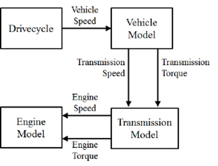
Unlike backwards-facing models (Figure 2), the speed trace is not “imposed” onto the vehicle model in forward-facing models, and therefore there will inevitably be a small margin of error between the actual vehicle speed and the speed trace. It is the role of the driver model to minimize this margin of error. This is similar to the role of a real-world test driver carrying out an emissions test for vehicle-type approval. Forward-facing models provide insight into the vehicle model's drivability, and it captures the limits of the physical system. It also makes control development and implementation on HIL systems easier. However, with the presence of multiple state equations in a typical forward-facing model, the vehicle speed (and subsequently drivetrain angular velocity) is computed via multiple state integration, resulting in the need to simulate smaller time steps. This results in longer simulation times when compared to backwards-facing models. Furthermore, resizing the powertrain will alter the dynamics of the system. This potentially requires the driver model to be re-tuned to maximize the performance of the system in areas such as fuel economy and longitudinal acceleration.
Backward Models
Backward models are calculated in a quasi-static manner. The inputs include vehicle conditions like velocity and acceleration, whereas the output is the force, torque, and power required at the source, i.e. the engine. They are simple and quick to use, making them ideal for quick computations and comparisons. They lack dynamics, and the method is mostly used to calculate simple fuel consumption and optimize energy management.

The ability of the vehicle model to meet the demands of the drive cycle is the principal assumption of a backwards-facing model. Based on the speed trace, the resultant force at the tire contact patch is calculated, where it is converted into wheel torque and propagated back to the ICE via the drivetrain, along with angular velocity. As a result, there is no driver model present. With both speed and torque imposed onto the powertrain components, a backwards-facing model can also be considered non-causal (physically non-realizable), as described by Hauer and Moore. During the optimization routine, the powertrain component sizing is determined by the ability of the component to address both the speed and torque imposed on the component (i.e., the power requirements). Backwards-facing models rely on efficiency maps that were created based on torque and speed data and are usually produced during steady-state real-world testing. This results in the calculation being relatively simpler than forward-facing models (essentially lookup tables instead of state equations), and can therefore be run over relatively larger time steps. Unfortunately, the very nature of using steady-state maps hinders the performance of backwards-facing models when it comes to representing dynamic effects.
Hybrid Electric Vehicles
we are going to go through different system architectures for Mild Hybrid Electric Vehicles (MHEV), looking into the positioning of the components on the vehicle, the possible control functions and advantages and disadvantages in terms of fuel efficiency and driveability.
Most of the vehicles in use worldwide are still powered by internal combustion engines (ICE), either gasoline/petrol or diesel. A Hybrid Electric Vehicle (HEV) has at least two sources of power for propulsion: the internal combustion engine and an electric motor.
There are three main reasons for which the automotive manufacturers are developing and selling HEVs:
- reduction of the CO2 emissions (by reduction of the fuel consumption)
- reduction of the exhaust gas toxic emissions
- improvement of the powertrain dynamics (by increasing total power and torque)
The powertrain of a HEV is quite complex because it contains all the components of an ICE vehicle plus most of the components of a pure electric vehicle (EV). Also, depending on the level of hybridization, it needs two energy sources, the fuel tank for the engine and a battery for the electric machine.
categories of hybrid vehicles are Micro, Mild, Full And Plug-In Hybrid Electric Vehicles.
By architecture, topology or configuration we understand the positioning of the main components of the hybrid electric system on the vehicle. Since the only mechanical link between the electrical system and the rest of the vehicle is done through the electric machine, the MHEV architecture is basically defined by the position of the electric machine and the type of connection with the powertrain / drivetrain (belt, integrated or gear mesh).
Types of Mild Hybrid Electric Vehicles (MHEV)
In this article we are going to go through different system architectures for Mild Hybrid Electric Vehicles (MHEV), looking into the positioning of the components on the vehicle, the possible control functions and advantages and disadvantages in terms of fuel efficiency and driveability.
To recall the different types of hybrid electric vehicles and what makes a mild hybrid electric vehicle, read the following articles:
- Understanding micro, mild, full and plug-in hybrid electric vehicles
- Mild Hybrid Electric Vehicle (MHEV) – introduction
By architecture, topology or configuration we understand the positioning of the main components of the hybrid electric system on the vehicle. Since the only mechanical link between the electrical system and the rest of the vehicle is done through the electric machine, the MHEV architecture is basically defined by the position of the electric machine and the type of connection with the powertrain / drivetrain (belt, integrated or gear mesh).
The 48V electrical system has become the industry standard for mild hybrid MHEV applications for several reasons:
- it’s relatively simple to integrate on a vehicle
- it’s modular, safe and compact
- the mass of the components is relatively small so the impact on the total weight of the vehicle is limited
- the system cost to performance (fuel efficiency, torque boost) ratio is very competitive
With the except of the crankshaft-mounted integrated starter generator (Honda IMA and Mercedes Benz BlueHybrid), all the mild hybrid vehicle architectures presented in this article are based on 48V systems.
The powertrain configuration of the MHEV system has significant impact on the performance and characteristics of the vehicle, in terms of:
- integration cost
- fuel efficiency
- dynamic performance (powertrain torque enhancement)
Automotive OEMs and automotive Tier 1 system suppliers are currently analyzing and evaluating several major powertrain architectures for MHEVs. The electric machine can be positioned, relative to the other powertrain components, in five major points:
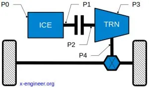
The brief description of the electric machine connection points is done in the table below.
| P0 | The electric machine is connected with the internal combustion engine through a belt, on the front end accessory drive (FEAD) |
| P1 | The electric machine is connected directly with the crankshaft of the internal combustion engine |
| P2 | The electric machine is side-attached (through a belt) or integrated between the internal combustion engine and the transmission; the electric machine is decoupled from the ICE and it has the same speed of the ICE (or multiple of it) |
| P3 | The electric machine is connected through a gear mesh with the transmission; the electric machine is decoupled from the ICE and it’s speed is a multiple of the wheel speed |
| P4 | The electric machine is connected through a gear mesh on the rear axle of the vehicle; the electric machine is decoupled form the ICE and it’s located in the rear axle drive or in the wheels hub |
Crankshaft mounted electric machine (P1)
The P1 architecture, with the electric machine connected directly to the crankshaft, is the solution adopted by Honda on their first generation Integrated Motor Assist (IMA) technology. The electric motor functions as a generator, during vehicle deceleration, as an engine starter, and as a motor (to assist the engine) during vehicle accelerations.

Image: MHEV P1 architecture – Integrated Starter Generator (ISG)
One of the biggest advantage of this solution is that the electric motor can provide higher torque than the BiSG, since there is no belt limitation (due to slip). However, since there is no speed / torque ratio between the electric machine and crankshaft, the torque requirements on the electric motor can be quite demanding.
wo examples of P1 MHEV architectures are:
- Honda Insight Hybrid 2009 (with Integrated Motor Assist technology)
- Mercedes Benz S400 Bluehybrid 2010.

Image: Integrated Motor Assist (IMA) for mild hybrid
Credit: Honda
For example, the main characteristics of the crankshaft-mounted electric machine for mild hybrid Honda Insight 2009 are summarized in the table below.
| Electric machine performance | Maximum torque (at crankshaft): up to 34 Nm Maximum power: 10 kW Efficiency: up to 94% |
| Hybrid modes (functions) | Idle Stop & Start Moving Stop & Start Engine load shift Torque assist (fill) Torque boost Sailing / Coasting Energy recuperation Brake regeneration |
| Advantages | Higher efficiency The 12V starter can be removed |
| Disadvantages | Output torque limited by the size of the electric machine Energy recuperation affected by engine friction losses High impact on existing vehicle architecture Higher overall cost of the electrical components Air cooling not possible for the electric machine |
| Overall characteristics | Torque Boosting Capability: High (if electric machine is capable) Electrical Energy Recuperation: Medium (due to engine losses) Driveability Improvements: Medium (depending on the torque capability of the electric machine) Electrical Creep / Drive: Possible (depending on the torque capability of the e-machine) Packaging: Difficult components integration (powertrain specially designed for this architecture) System Efficiency: High (no gear mesh or belt losses) |
Run the “Project2_InitFile.m” Matlab script
%%%%%%%%%%%%%%%%%%%%%%%%%%%%%%%%%%%%%%%%%%%%%%%%%%%%%%%%%%%%%%%%%%%%%
%% Skill-Lync -> Hybrid Drives Development
% Project 1 - Conventional Vehicle Model
% By - Ullekh Gambhira

% Description:

%% Initialization File
% Initialization file for loading the variables for the Conventional vehicle simulation model

%% Vehicle Parameters
M = 1500;       % Vehicle weight [kg]
Cr = 0.015;     % Rolling resistance coefficient
Rw = 0.35;      % Rolling radius [m]
Cd = 0.33;      % Drag coefficient
Af = 2;         % Frontal area [m2]
rhoa = 1.225;   % Air density [kg/m3]
Vwind = 0;      % Wind velocity [kmph]
g = 9.81;       % Gravitational acceleration [m/s2]
theta = 0;      % Slope [deg]
myu_road_tire = 1; % Coefficient of friction between tire - road interface

%% Powertrain Parameters
FDR = 3.73;                         % Final Drive Ratio / Diff Ratio
DiffEff = 0.99;                     % Differential efficiency (assumed independent of operating conditions)

NumGear = 4;                        % Number of gears in transmission
TransGear = [1:NumGear];            % Transmission Gears
TransRatio = [3.06, 1.62, 1, 0.7];  % Corresponding Transmission ratios
TransEff = 0.90;                    % Transmission efficiency (assumed independent of operating conditions)

TC_SR = [0, .5, .6, .7, .8, .87, .92, .94, .96, .97, 1];   % Torque Converter Speed Ratio (Matlab default) -> TurbSpd/PumpSpd
TC_TR = [2.232, 1.5462, 1.4058, 1.2746, 1.1528, 1.0732, 1.0192, 1, 1, 1, 1];   % Torque Converter Torque Ratio (Matlab default) -> TurbTrq/PumpTrq
TC_Cf = 1e-4 * [.72558, .66322, .63463, .59042, .51331, .4144, .29287, .22444, .12186, .04386, 0]; % Torque Converter Capacity Factor (Matlab default) -> PumpTrq/PumpSpd^2 [Nm/rpm^2]

load Vehicle_Data/Engine_data_1_9L_Saturn_95kW
load Vehicle_Data/Trans_Shift_map
load Vehicle_Data/EM_Honda_Insight_10kW
load Vehicle_Data/ESS_NiMH6


ESS_init_soc = 0.8;
ESS_soc_max = 0.9;
ESS_soc_min = 0.6;


%% Driver Parameters
Kp = 10;                    % P gain for driver PI model
Ki = 1;                     % I gain for driver PI model
Drive_Cycle_Select = 2;     % Drive cycle selection

Drive_Cycle_Select =input('Enter Drive cycle Number =');

% Drive cycle values in m/s

if Drive_Cycle_Select == 1
    load DriveCycles/UDDS;

elseif Drive_Cycle_Select == 2
    load DriveCycles/HWFET;

elseif Drive_Cycle_Select == 3
    load DriveCycles/FTP;

elseif Drive_Cycle_Select == 4
    load DriveCycles/US06;

elseif Drive_Cycle_Select == 5
    load DriveCycles/NEDC;

elseif Drive_Cycle_Select == 6
    load DriveCycles/WLTP;

end

time_end = cyc_time(end);
vel_end = cyc_vel(end);
The initial MATLAB file is loaded.
All variables from the file created in the workspace.
Giving input to the initial file from the command window.
Choose the required Drive cycle number and give input to the initial file.
The next step is to create the Simulink model of the P1 hybrid vehicle according to project requirements.
- The Drive Cycle can be selected from this MATLAB Script, By changing the variable Drive _Cycle _Select to,
- UDDS
- HWFET
- FTP
- USO6
- NEDC
- WLTP
Simulink Model For P1 Hybrid Vehicle.
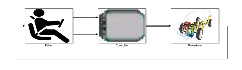
The Simulink model consists of three main subsystems: Driver, Controller and Powertrain, as shown in Figure 4. The Driver subsystem generates the accelerator and brake pedal outputs to match the desired and actual vehicle speed. The Controller block represents the electronic control units, which generate the desired engine torque, transmission gear and brake torque based on the driver inputs. The Powertrain subsystem represents the vehicle consisting of all vehicle components that input the control signals from the Controller and provides actual vehicle motion characteristics.
Sub-systems and blocks mention below.
1. Driver
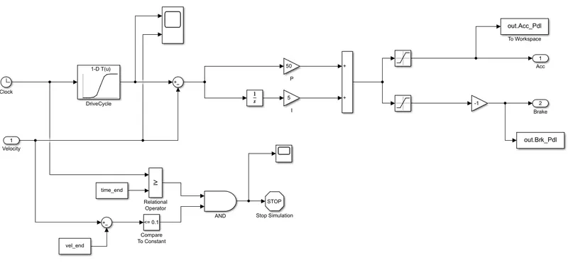
The Driver model block is a basic PI controller that generates accelerator and brake pedal outputs to match the desired and actual vehicle speeds. The PI controller minimizes the error between the required vehicle speed and the actual speed of the vehicle.
2. Controler
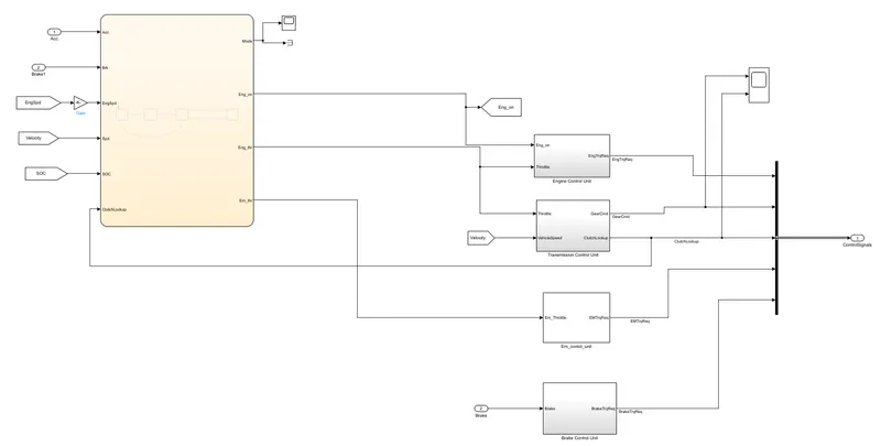
The controller block is the brain of the vehicle. It contains the ECU. Based on the driver inputs, the controller block generates the output and this is fed into the powertrain block of the system. The Controller block has a Mode Selection chart, created for the hybrid architecture, to choose the operating mode of the vehicle based on the driver inputs. Based upon this, the engine control unit, the transmission control unit, and the motor control unit generate output. This output feeds into the powertrain unit. The power train unit generates output according to the control unit feedback. And obtain the efficient operation of the vehicle.
The subsystems of the Controller unit are as follows.
i.Engine Control unit
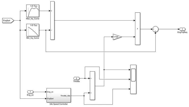
An engine control unit (ECU), also commonly called an engine control module (ECM), is a type of electronic control unit that controls a series of actuators on an internal combustion engine to ensure optimal engine performance. It does this by reading values from a multitude of sensors within the engine bay, interpreting the data using multidimensional performance maps (called lookup tables), and adjusting the engine actuators. Before ECUs, air–fuel mixture, ignition timing, and idle speed were mechanically set and dynamically controlled by mechanical and pneumatic means.
Ideal Speed controler
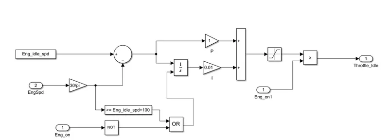
The Idle Speed Controller is a PI Controller where the engine speed and the idle speed of the engine are compared. The error is then multiplied with constant P and the integrated error is multiplied with constant I. Here we add the product block for the cut to give a signal to the on-off engine to close the throttle and reduce fuel consumption during the ideal condition.
ii.Transmission control unit
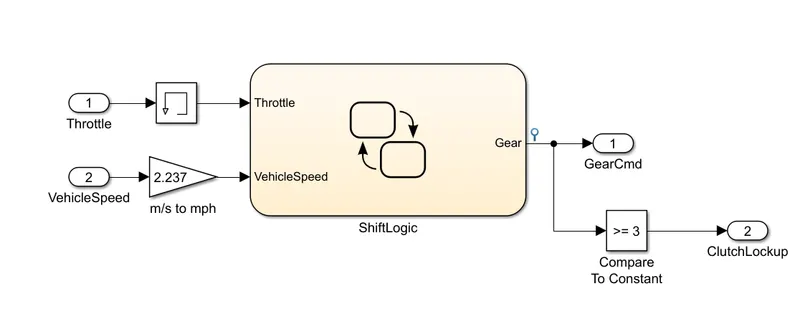
It uses a state logic and provided the current gear of the vehicle. The state is defined by comparing the throttle signal and vehicle speed. The ShiftLogic is the logic control block for defining the gear.
A transmission control unit (TCU), also known as a transmission control module (TCM), or a gearbox control unit (GCU), is a type of automotive ECU that is used to control electronic automatic transmissions. Similar systems are used in conjunction with various semi-automatic transmissions, purely for clutch automation and actuation. A TCU in a modern automatic transmission generally uses sensors from the vehicle, as well as data provided by the engine control unit (ECU), to calculate how and when to change gears in the vehicle for optimum performance, fuel economy and shift quality.
Here we add to compare to the constant block for lockup of the clutch after 3rd gear for better fuel efficiency.
ShiftLogic Block
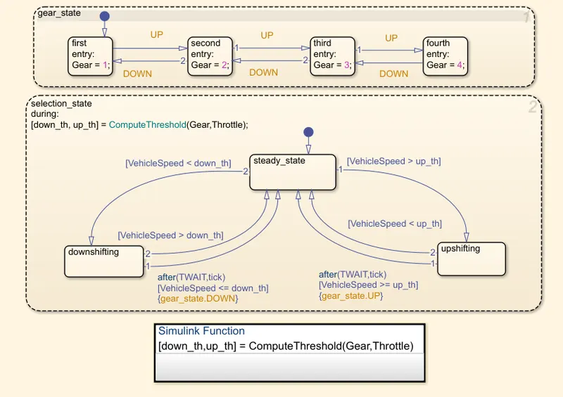
The gear_state is defined between 4 states as the vehicle has four gears in total. The UP and DOWN values are calculated using another state selection_state. When in the selection_gear state, a function ComputeThreshold is calculated where the inputs are Gear and Throttle. The output will be down_th and up_th for the function which is speed limits. The outputs from the function are fed in, then the downshift and upshift are done based on vehicle speed and the parameter inputs from the Matlab file Trans_Shift_map.
ComputeThreshold function
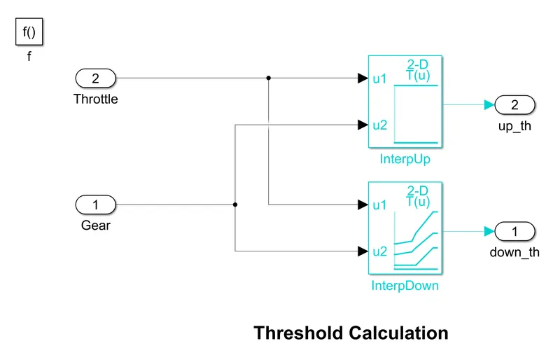
The function uses lookup tables to find the transmission shifts and provides two outputs which feed the selection_state.
iii. Electric Motor Control Unit
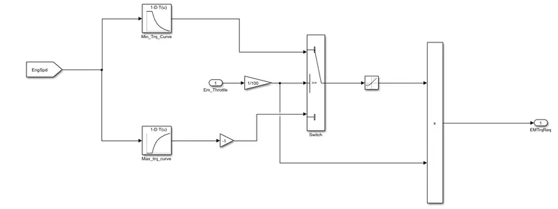
Motor Control Unit (MCU) is an electronic module that interfaces between the batteries and motor to control the electric vehicle’s speed and acceleration based on throttle input. The controller transforms the battery’s direct current into alternating current and regulates the energy flow from the battery.
In this block On the basis of engine speed requirement, the required electric motor torque is calculated and fed to the electric motor block.
iv. Brack Control Unit
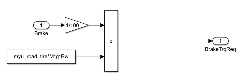
The Brake pedal signal from the Driver block is multiplied by the maximum friction, which gives the maximum braking torque. The gain block is used to convert the actual value in percentage.
3. Powertrain Block
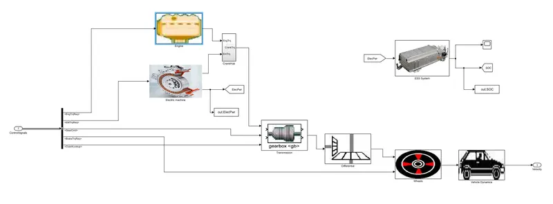
- The powertrain model includes all the components that convert the power of the engine into vehicle motion.
- This includes the engine, Battery Pack, Electric Motor, Crank Hub, Transmission, Differential, Wheels and the vehicle
body dynamics subsystems. - The control signals from the control model are transmitted via a bus to the corresponding blocks in the
powertrain model.
i.)Energy Storage System(Battery)
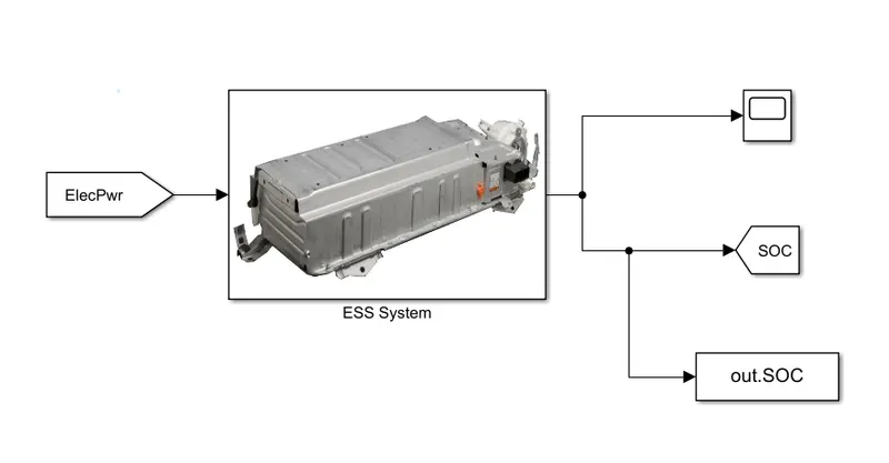
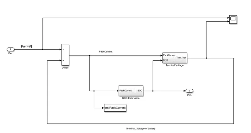
Here for Ess System Electric power is in input and SOC of battery is output.
In the ESS block, there is a sub-block of SOC estimate and terminal voltage block.
The required power for an electric motor is given input to Ess block according to that voltage current and SOC of battery find out.
SOC Estimation Block
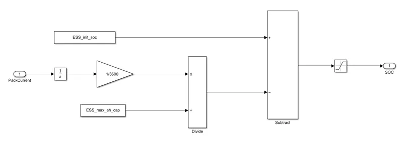
Pack current in Ampere is converted to AmpHour and divides with Max Capacity and adds with the Initial soc to determine the SOC of the battery at each instance, the SOC value is limited between 0 to 1.
Terminal Voltage Block
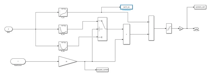
- Open circuite voltage and internal resistance are determined by 1D lookup tables, and pack current determined using the model.
- Calculate the voltage using formula V=IR and this voltage is subtracted from open circute voltage.
- Terminal voltage is calculated using number of cell in battey pack to be multiply with cell voltage.
- The specified values are sent back to the workspace using the Two Workspace block and can used for post processing.
ii.)Engine Block
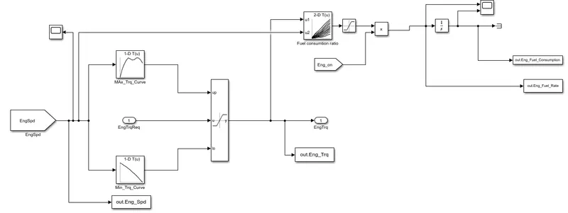
- Based on the Engine speed The required torque from the controller is saturated between Max torque curve and min torque curve and passes the Engine torque to the Transmission block.
- The 2D lookup table is used to calculate the fuel flow rate based on engine speed and engine torque. The fuel flow rate is then integrated to find the fuel consumption.
- Estimated fuel flow rate, fuel consumption, engine torque and engine speed are passed to the MATLAB workspace using the to-workspace block.
- Engine fuel flow rate and Fuel consumption are scoped.
iii.) Electric Motor Model
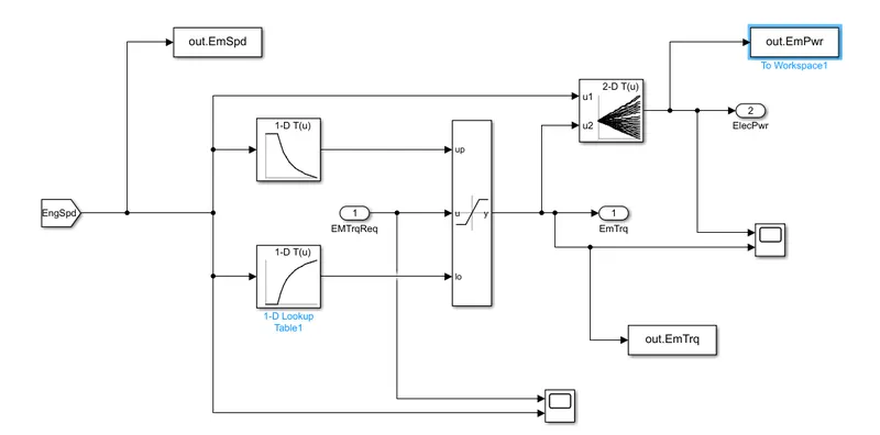
- Based on the Engine speed The required EM torque from the controller is saturated between Max EM torque
curve and max EM torque Generation curve and passes the EM torque to the Crank Hub. - The 2D lookup table is used to calculate the Input Electric Power to the Motor based on EM speed and EM torque.
iv) Crank Hub
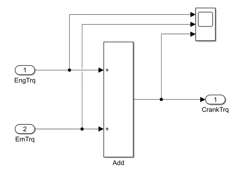
- Crank Hub adds up the EM torque and the Engine torque and pass it to the transmission block as the crank
torque.
V)Transmission Block
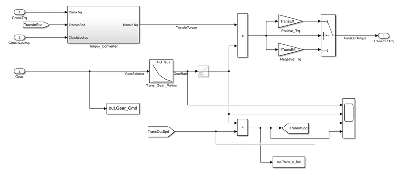
- The Crank is connected to the automatic transmission via a torque converter. The output of the transmission is
connected to the differential. - New Clutch LockUp feature is adding to this Hybrid version.
Torque convertor
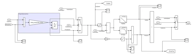
- Torque converter defines the pumb and turbine torque by the clutch lock-up status, and the combination gives
us the desired transmission torque.
vi) Differential
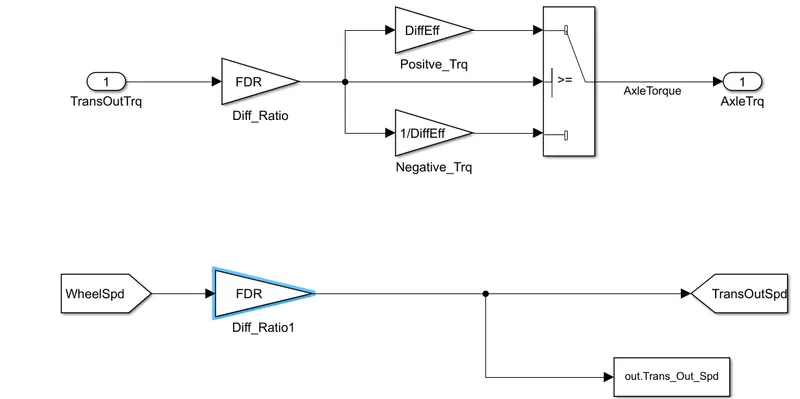
- The transmission output torque is multiplied by the differential ratio and differential efficiency in this block and the torque is transmitted to the wheel as the axle torque.
vii) Wheel Block
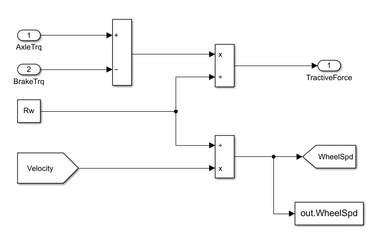
- The brake torque from the control model is subtracted from the Axle torque and divides from the rolling radius to determine the Tractive force.
- The Wheel speed is calculated from the vehicle velocity and saved in the workspace.
viii) Vehicle Dynamics
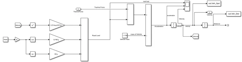
- The longitudinal dynamics of the vehicle along with the road load is represented in the 'Vehicle Dynamics' block.
- Tractive Force and Road loads are used to calculate the vehicle velocity.
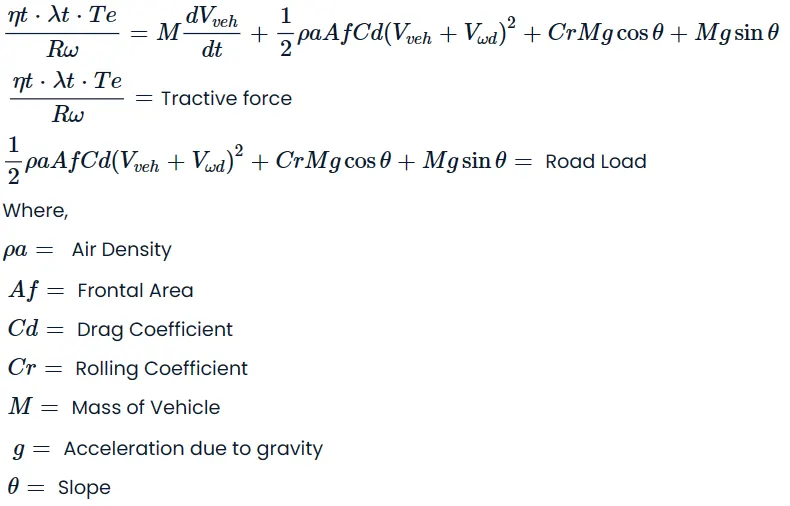
- The variables are loaded on the workspace using MATLAB script.
- The Acceleration, Velocity and Distance travelled are Calculation and stored in the workspace.
Processing file
%% Post-Processing File
% Skill-Lync -> Hybrid Drives Development
% Project 2 - P1_Hybrid_Vehicle_Model
% By - Ajay Ghanwat
%% Renaming variables
Time = out.tout;
Acc_Pdl = out.Acc_Pdl;          % Accelerator pedal [%]
Brk_Pdl = out.Brk_Pdl;          % Brake pedal [%]
Gear_Cmd = out.Gear_Cmd;        % Transmission gear
Trans_In_Spd = out.Trans_In_Spd*30/pi;  % Transmission input speed [rpm]
Trans_Out_Spd=out.Trans_Out_Spd*30/pi;% Transmission output speed [rpm]
Eng_Trq = out.EngTrq;          % Engine brake torque [Nm]
Eng_Spd = out.Eng_Spd*30/pi;    % Engine speed [rpm]
Eng_Fuel_Consump = out.Eng_Fuel_Consumption;    % Engine fuel consumption [g]
Veh_Dist = out.Veh_Dist/1000;   % Distance traveled by vehicle [km]
Veh_Spd = out.Veh_Spd*18/5;     % Vehicle speed [kmph]
Wheel_Speed = out.WheelSpd;     % Wheel speed [kmph]
Eng_Fuel_Rate = out.Eng_Fuel_Rate; % Engine fuel rate [%]
EM_Speed = out.EmSpd*18/5;        % Electric Motor Speed
EM_Power = out.EmPwr;            % Electric Motor Power
EM_Torque = out.EmTrq;           % Electric Motor Torque
Ter_Volt = out.term_volt;        % Terminal Voltage of battery
Soc = out.SOC;                    % State Of Charge
Pack_Current = out.pack_current;   %Pack current of battery
Eng_Trq=Eng_Trq.Data(:,1);
Eng_Spd=Eng_Spd.Data(:,1);
%% Data Analysis
Eng_Pwr = Eng_Spd.*pi./30.*Eng_Trq./1000;   % Engine brake power [kW]
rho_petrol = 0.7197;                    % Density of petrol [kg/L]
kmpl = Veh_Dist(end)/(Eng_Fuel_Consump(end)/1000/rho_petrol);    % Fuel economy [kmpl]


%% Plotting vehicle characteristics time trace transmission IN/OUT and Wheel Speed
figure(1)
hold on
grid on
plot(Time, Trans_In_Spd, 'linewidth', 1, 'Color', 'black');
plot(Time, Trans_Out_Spd, 'linewidth', 1, 'Color', 'red');
plot(Time, Wheel_Speed, 'linewidth',1, 'color', 'blue')
ylabel('Speed [rpm]')
xlabel('Timem [s]')
xlim([0, Time(end)]);
ylim([0, 6000]);
legend('Trans Input','Trans Output','Wheel Speed');

%% Plotting Engine speed, Engine Torque, Engine Power,Engine fuel rate,Engine fuel consumption wrt Time
figure(2)
subplot(4,1,1)
plot(Time,Eng_Trq,'linewidth',1,'color','black')
%xlim([0, Time(end)]);
xlabel('Time [s]')
ylabel('Torque [Nm]')
legend('Engine Torque')
grid on

subplot(4,1,2)
plot(Time,Eng_Pwr,'linewidth',1,'color','blue')
xlim([0, Time(end)]);
xlabel('Time [s]')
ylabel('Power [KW]')
legend('Engine Power')
grid on

subplot(4,1,3)
plot(Time,Eng_Fuel_Rate,'linewidth',1,'color','red')
xlim([0, Time(end)]);
xlabel('Time [s]')
ylabel('Fuel Rate [%]')
legend('Engine Fuel Rate')
grid on

subplot(4,1,4)
plot(Time,Eng_Fuel_Consump,'linewidth',1,'color','green')
xlim([0, Time(end)]);
xlabel('Time [s]')
ylabel('Fuel Consumption')
legend('Engine Fuel Consumption')
grid on

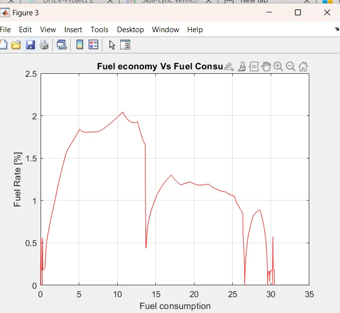
% Plotting fuel economy Vs Engine Fuel consumption
figure(3)
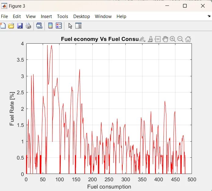
plot(Eng_Fuel_Consump,Eng_Fuel_Rate,'color','r')
xlabel('Fuel consumption')
ylabel('Fuel Rate [%]')
title('Fuel economy Vs Fuel Consumption')
grid on

%% Potting Accelerator pedal, Brake pedal and gear command with respect to time
figure(4)
subplot(2,1,1)
hold on
plot(Time, Acc_Pdl, 'linewidth', 1, 'Color', 'black');
plot(Time, Brk_Pdl, 'linewidth', 1, 'Color', 'red');
ylabel('Pedal [%]')
xlabel('Time [s]');
xlim([0, Time(end)]);
grid on
legend('Accel','Brake');
title('Acceleration & Brake Pedal wrt Time')

subplot(2,1,2)
plot(Time, Gear_Cmd, 'linewidth', 1, 'Color', 'black');
xlim([0, Time(end)]);
xlabel('Time [s]');
ylabel('Gear');
grid on
title('Gear command wrt Time')

% Plotting gear command vehicle desired with actual speed
figure(5)
subplot(2,1,1)
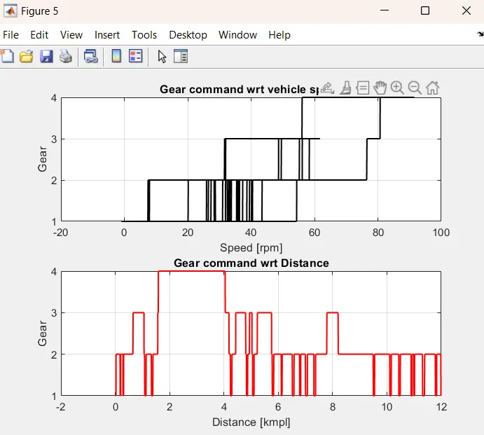
plot(Veh_Spd, Gear_Cmd, 'linewidth', 1, 'Color', 'black');
xlabel('Speed [rpm]');
ylabel('Gear');
grid on
title('Gear command wrt vehicle speed')

subplot(2,1,2)
plot(Veh_Dist, Gear_Cmd, 'linewidth', 1, 'Color', 'red');
xlabel('Distance [kmpl]');
ylabel('Gear');
grid on
title('Gear command wrt Distance')

%% Plotting engine operating points on engine fuel map
figure('Name','Engine Operating Points');
hold on
grid on
title('Engine Operating Points','fontsize',12);
p1=plot(Eng_map_spd*30/pi,Eng_max_trq,'linewidth',2,'color','r');
p2=line([Eng_map_spd(end)*30/pi Eng_map_spd(end)*30/pi],[0 Eng_max_trq(end)]);
set(p2,'linewidth',1,'linestyle','--','color','k');
p3=line([Eng_map_spd(1)*30/pi Eng_map_spd(1)*30/pi],[0 Eng_max_trq(1)]);
set(p3,'linewidth',1,'linestyle','--','color','k');
[c,h] = contour(Eng_map_spd'*30/pi,Eng_map_trq,Eng_fuel_map');
clabel(c,h);
xlabel('Engine Speed [rpm]');
ylabel('Engine Torque [Nm]');
title('Engine Fuel Consumption Map [g/s]');
legend([p1 p3],{'Max Curve','Operating Points'});
axis([Eng_map_spd(1)*30/pi Eng_map_spd(end)*30/pi 0 Eng_map_trq(end)]);

%% State of Charge, Pack Current, And Terminal Voltage with respect to Time
figure(6)
subplot(3,1,1)
plot(Time,Pack_Current,'linewidth',1,'color','black')
xlim([0, Time(end)]);
xlabel('Time [s]')
ylabel('Current [W]')
legend('Pack Current')
grid on

subplot(3,1,2)
plot(Time,Soc,'linewidth',1,'color','blue')
xlim([0, Time(end)]);
xlabel('Time [s]')
ylabel('Charging [%]')
legend('State Of Charge')
grid on

subplot(3,1,3)
plot(Time,Ter_Volt,'linewidth',1,'color','red')
xlim([0, Time(end)]);
xlabel('Time [s]')
ylabel('Voltage [V]')
legend('Terminal Voltage')
grid on

%% Motor Speed, Torque, Motor input power with respect to Time
figure(7)
subplot(3,1,1)
plot(Time,EM_Power,'linewidth',1,'color','black')
xlim([0, Time(end)]);
xlabel('Time [s]')
ylabel('Power [W]')
legend('Electric Motor Power ')
grid on

subplot(3,1,2)
plot(Time,EM_Torque,'linewidth',1,'color','blue')
xlim([0, Time(end)]);
xlabel('Time [s]')
ylabel(' Torque [Nm]')
legend('Electric Motor Torque')
grid on

subplot(3,1,3)
plot(Time,EM_Speed,'linewidth',1,'color','red')
xlim([0, Time(end)]);
xlabel('Time [s]')
ylabel('Speed [Rpm]')
legend('Electrical Motor Speed')
grid on

%% Plotting EM Operating Points on motor input power Map
figure('Name','Electric Motor Operating Points');
hold on
grid on
title('Electric Motor Operating Points','fontsize',12);
p1=plot(EM_map_spd*30/pi,EM_max_trq,'linewidth',2,'color','r');
p2=line([EM_map_spd(end)*30/pi EM_map_spd(end)*30/pi],[0 EM_max_trq(end)]);
set(p2,'linewidth',1,'linestyle','--','color','k');
p3=line([EM_map_spd(1)*30/pi EM_map_spd(1)*30/pi],[0 EM_max_trq(1)]);
set(p3,'linewidth',1,'linestyle','--','color','k');
[c,h] = contour(EM_map_spd'*30/pi,EM_map_trq,EM_inpwr_map');
clabel(c,h);
xlabel('Motor Speed [rpm]');
ylabel('Motor Torque [Nm]');
title('Motor Input Power Map [g/s]');
legend([p1 p3],{'Max Curve','Operating Points'});
axis([EM_map_spd(1)*30/pi EM_map_spd(end)*30/pi 0 EM_map_trq(end)]);
%%
fprintf('Fuel Economy = %9.3f\n',kmpl(end));
Results
The P1 hybrid vehicle model was run for different drive cycles and got the results for the required parameters of the HEV vehicles.
Compare these results with the existing conventional vehicle model.
UDDS Drive Cycle
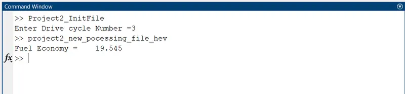
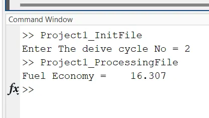
Fuel Economy
For p1 hybrid
For conventional Vehicle
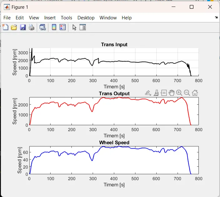
Graph of Transmission input speed, transmission output speed and Wheel Speed.
Graph of Engine Torque, Engine Power, Engine Fuel Rate, and Engine fuel consumption.
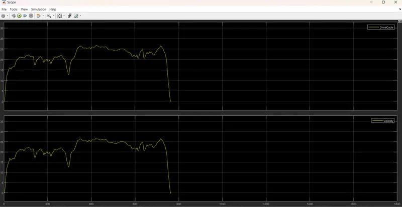
HWFET Drive Cycle
for P1 HEV
For conventional
Conclusion :
The Various performance of characteristics and operating points of the UDDS drive cycle and HWFET drive cycle are analysed and graphs are plotted.
- Time trace for engine, Transmission input, Transmission output and wheel speed with respect to time.
- Engine torque, Engine power, Fuel rate and Fuel consumption with respect to time.
- Accelerator and brake pedal, gear command and vehicle desired, actual speed, vehicle distance with respect to time.
- Engine operating points on the engine fuel map with respect to time
- Motor speed, Torque, and Motor input power with respect to time.
- Pack voltage, Current and State of charging with respect to time.
- The motor operating points on the motor input power map with respect to time.
and also it comparing with HWFET drive cycle and their numbers also compared.
Google Drive link
https://drive.google.com/drive/folders/10HumF6kyrBqvsx9W0EqaUjgsJsuRjoh5?usp=share_link