Project 1 - Parsing NASA thermodynamic data
Aim-1. Write a function that extracts the 14 co-efficients and calculates the enthalpy, entropy and specific heats for all the species in the data file.
2. Calculate the molecular weight of each species and display it in the command window.
3. Plot the Cp, Enthalpy and Entropy for the local temperature range (low temperature : high temperature) specific for each species.
4. Save the plots as images with appropriate names and dump them in separate folders for each species with suitable name. All these should be generated automatically.
5. The main program that you will submit will just take the "THERMO.dat" file as an input and generate Cp, H and S plots.
6. Please write a detailed report to describe your logic.
Description
Ideal Gas Thermodynamic Properties in Chemkin Format Thermodynamic properties for ideal gases are tabulated in a variety of locations in Chemkin format. This format involves two sets of 7 constants a1 through a7. These constants are fits to specific heat, enthalpy, and entropy data (or calculations) according to the following formulae:
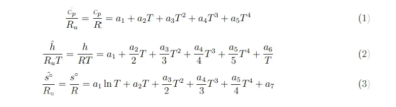
Cp= specific heat
R=Universal gas constant
h=enthalpy
s=entropy
T=temperature
Note that all the parameters on the left-hand side of equations (1) through (3) are dimensionless. Three temperatures are given on the first line of the data, Tlow, Thigh, and Tmid. Usually, these values are 300, 5000, and 1000 K respectively. The first set of parameters a1 through a7 applies for the high temperature range (Tmid through Thigh), while the second set applies for the low temperature range (Tlow through Tmid).
1) Write a function that extracts the 14 co-efficients and calculates the enthalpy, entropy and specific heats for all the species in the data file.
%%%%%         Parsing NASA thermodynamic data         %%%%%

close
clear
clc

f1=fopen('THERMO.dat','r'); % Read the data file
fgetl(f1);                  % skip the line

% Reading the Header information in data file

tline=fgetl(f1);
A=strsplit(tline,' ');
globl_low_temp=str2num(A{2}); % convert string to number
globl_mid_temp=str2num(A{3}); % convert string to number
globl_high_temp=str2num(A{4});% convert string to number

% Skip next 3 line in data file
for i=1:3
fgetl(f1);
end
% Reading the species Data (53 Species)
for i=1:53     % for loop is used to read 53 species and it's data
    header=fgetl(f1);

    x=strsplit(header,' ');
    species_name=(x{1});
    z=length(x);
% getting temperature value from next header information
    local_low_temp=str2double(x{z-3});
    local_high_temp=str2double(x{z-2});
    local_mid_temp=str2double(x{z-1});

    t1=local_low_temp;
    t2=local_mid_temp;
    t3=local_high_temp;

    %%Collect the 1st line coefficient(a1 to a5)
    tline_1=fgetl(f1);

    a=strfind(tline_1,'E'); % strfind command is used to find position of E in string
    a1=tline_1(1:a(1)+3);   % according to position of E, read the number befor E and after E.
    a1=str2double(a1);

    a2=tline_1(a(1)+4:a(2)+3);
    a2=str2double(a2);

    a3=tline_1(a(2)+4:a(3)+3);
    a3=str2double(a3);

    a4=tline_1(a(3)+4:a(4)+3);
    a4=str2double(a4);

    a5=tline_1(a(4)+4:a(5)+3);
    a5=str2double(a5);

 %%Collect the 1st line coefficient(a6 to a10)
    tline_2=fgetl(f1);
    b=strsplit(tline_2,' ');
    b=strfind(tline_2,'E');

    a6=tline_2(1:b(1)+3);
    a6=str2double(a6);

    a7=tline_2(b(1)+4:b(2)+3);
    a7=str2double(a7);

    a8=tline_2(b(2)+4:b(3)+3);
    a8=str2double(a8);

    a9=tline_2(b(3)+4:b(4)+3);
    a9=str2double(a9);

    a10=tline_2(a(4)+4:a(5)+3);
    a10=str2double(a10);

  %%Collect the 1st line coefficient(a11 to a14)
    tline_3=fgetl(f1);
    c=strfind(tline_3,'E');

    a11=tline_3(1:c(1)+3);
    a11=str2double(a11);

    a12=tline_3(c(1)+4:c(2)+3);
    a12=str2double(a12);

    a13=tline_3(c(2)+4:c(3)+3);
    a13=str2double(a13);

    a14=tline_3(c(3)+4:c(4)+3);
    a14=str2double(a14);

% creating folder to save data of species i.e plots
 mkdir(['D:\mtlab\study\file_parsing\Nasa thermo data\images\',species_name]);


   T=linspace(t1,t3,1000); %create temperature array
   R=8.314;               % universal gas constant.

   %%calculate array of specific heat,enthalpy and entropy,
   for j=1:length(T);

   %Temperature is asign to coefficients
   % a1 to a7 are high temperature coefficients
   if T(j)>t2                               % if loop is used here t2 is mid temperature
       Cp=(a1+a2.*T+a3.*T.^2+a4.*T.^3+a5.*T.^4)*R;
       H=(a1+(a2.*T)/2+(a3.*T.^2)/3+(a4.*T.^3)/4+(a5.*T.^4)/5+(a6./T))*R.*T;
       S=a1.*log(T)+a2.*T+(a3.*T.^2)/2+(a4.*T.^3)/3+(a5.*T.^4)/4+a7;
   else
       % a8 to a14 are low temperature coefficients
        Cp=(a8+a9.*T+a10.*T.^2+a11.*T.^3+a12.*T.^4)*R;
       H=(a8+(a9.*T)/2+(a10.*T.^2)/3+(a11.*T.^3)/4+(a12.*T.^4)/5+(a13./T))*R.*T;
       S=a8.*log(T)+a9.*T+(a10.*T.^2)/2+(a11.*T.^3)/3+(a12.*T.^4)/4+a14;

   end

end
3. Plot the Cp, Enthalpy and Entropy for the local temperature range (low temperature : high temperature) specific for each species.
     %plotting graphs of Cp,H,S Vs T

figure(1)
plot(T,Cp,'linewidth',2);
title(species_name);
xlabel('Temperature[K]');
ylabel('Specific Heat[J/Kg K]');


figure(2)
plot(T,H,'linewidth',2);
title(species_name);
xlabel('Temperature[K]');
ylabel('Enthalpy[kj/mol]');

figure(3)
plot(T,S,'linewidth',2);
title(species_name);
xlabel('Temperature[K]');
ylabel('Entropy[J/K]');


%change the directory and saving the plots
saving=(['D:\mtlab\study\file_parsing\Nasa thermo data\images\',species_name]);
cd(saving);
saveas(1,'Specific Heat','jpg');
saveas(2,'Enthalpy','jpg');
saveas(3,'Entropy','jpg');
2. Calculate the molecular weight of each species and display it in the command window.
% calculating the molecular weight of each species

elements=['H','C','O','N','AR','S'];
atomic_weight=[1.0079 12.0107 15.9994 14.0067 39.948 32.065];%Respective atomic weight of main species
 molecular_weight=0; % consider
 for l=1:length(species_name)
 for m=1:length(atomic_weight)

if strcmp(species_name(l),elements(m))  % strcmp command used to compaire the element and species in data
    molecular_weight=molecular_weight+atomic_weight(m) %to calculate molecular weight
    an=m; %consider
end
end

 n=str2num(species_name(l)) %molecul contain number of atoms so that for calculating molecular weight use if loop
 if n>1
     molecular_weight=molecular_weight+atomic_weight(an)*(n-1);
 end
 end
 sprintf('molecular_weight of %s:%f u',species_name,molecular_weight)% print the molecular weight of each species

end


fclose(f1)    %closing the data file
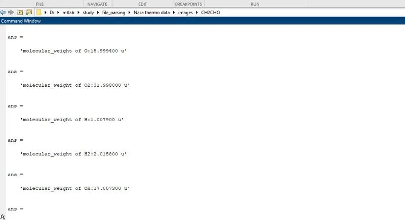
Here attached screenshot of molecular weight of all species in data file.
Here attached screenshot of the folder containing plot of Cp,H,S Vs T of all species.

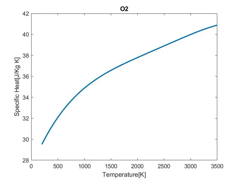
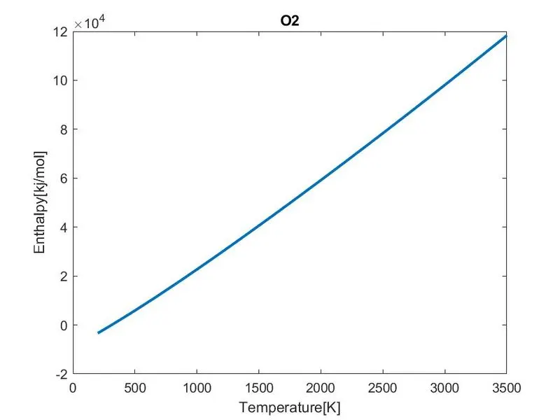
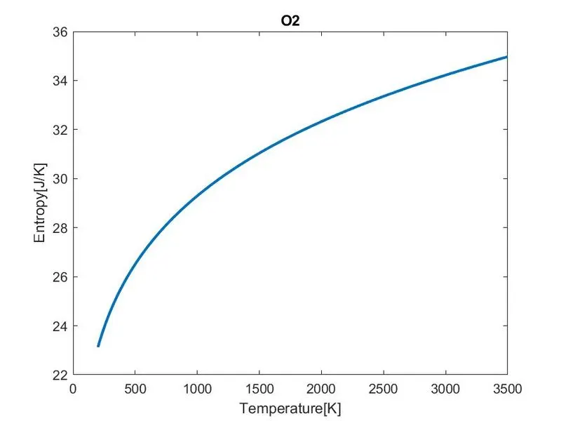
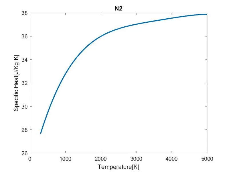
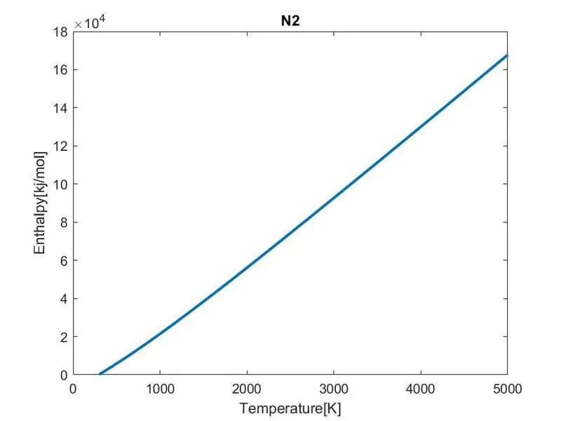
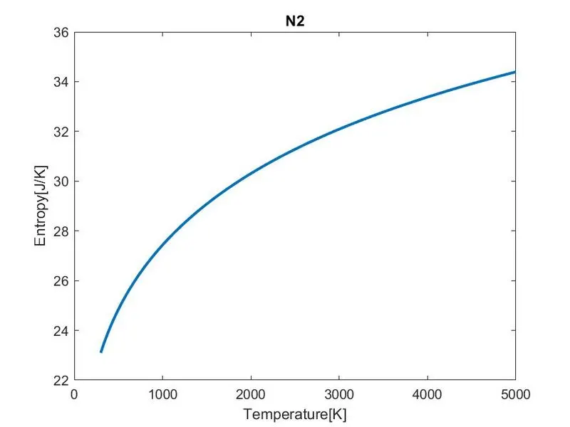
Attaching here plots of O2,N2,CO2
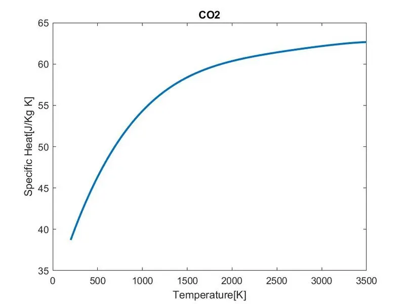
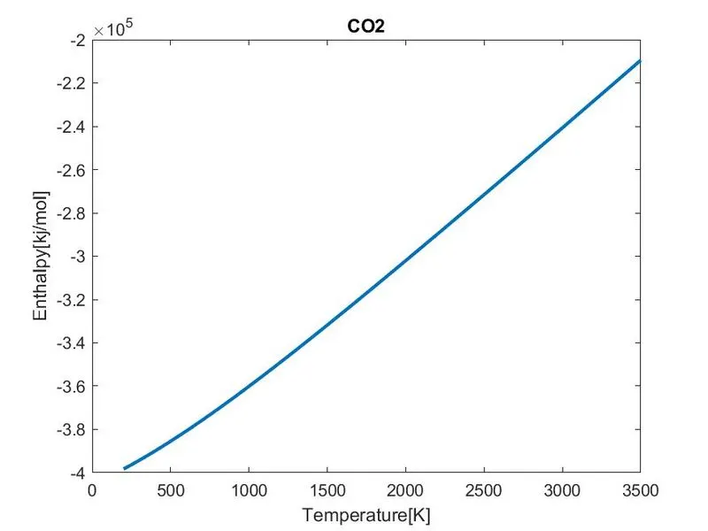
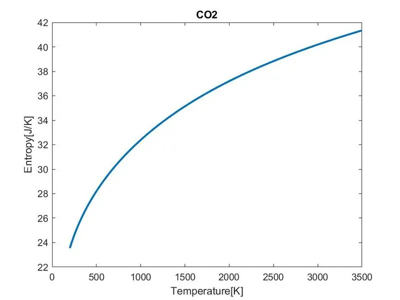
Full continuo
us code for NASA file parsing
Step wise CODE Explanation
%%%%%         Parsing NASA thermodynamic data         %%%%%

close
clear
clc

f1=fopen('THERMO.dat','r'); % Read the data file
fgetl(f1);                  % skip the line

% Reading the Header information in data file

tline=fgetl(f1);
A=strsplit(tline,' ');
globl_low_temp=str2num(A{2}); % convert string to number
globl_mid_temp=str2num(A{3}); % convert string to number
globl_high_temp=str2num(A{4});% convert string to number

% Skip next 3 line in data file
for i=1:3
fgetl(f1);
end
% Reading the species Data (53 Species)
for i=1:53     % for loop is used to read 53 species and it's data
    header=fgetl(f1);

    x=strsplit(header,' ');
    species_name=(x{1});
    z=length(x);
% getting temperature value from next header information
    local_low_temp=str2double(x{z-3});
    local_high_temp=str2double(x{z-2});
    local_mid_temp=str2double(x{z-1});

    t1=local_low_temp;
    t2=local_mid_temp;
    t3=local_high_temp;

    %%Collect the 1st line coefficient(a1 to a5)
    tline_1=fgetl(f1);

    a=strfind(tline_1,'E'); % strfind command is used to find position of E in string
    a1=tline_1(1:a(1)+3);   % according to position of E, read the number befor E and after E.
    a1=str2double(a1);

    a2=tline_1(a(1)+4:a(2)+3);
    a2=str2double(a2);

    a3=tline_1(a(2)+4:a(3)+3);
    a3=str2double(a3);

    a4=tline_1(a(3)+4:a(4)+3);
    a4=str2double(a4);

    a5=tline_1(a(4)+4:a(5)+3);
    a5=str2double(a5);

 %%Collect the 1st line coefficient(a6 to a10)
    tline_2=fgetl(f1);
    b=strsplit(tline_2,' ');
    b=strfind(tline_2,'E');

    a6=tline_2(1:b(1)+3);
    a6=str2double(a6);

    a7=tline_2(b(1)+4:b(2)+3);
    a7=str2double(a7);

    a8=tline_2(b(2)+4:b(3)+3);
    a8=str2double(a8);

    a9=tline_2(b(3)+4:b(4)+3);
    a9=str2double(a9);

    a10=tline_2(a(4)+4:a(5)+3);
    a10=str2double(a10);

  %%Collect the 1st line coefficient(a11 to a14)
    tline_3=fgetl(f1);
    c=strfind(tline_3,'E');

    a11=tline_3(1:c(1)+3);
    a11=str2double(a11);

    a12=tline_3(c(1)+4:c(2)+3);
    a12=str2double(a12);

    a13=tline_3(c(2)+4:c(3)+3);
    a13=str2double(a13);

    a14=tline_3(c(3)+4:c(4)+3);
    a14=str2double(a14);

% creating folder to save data of species i.e plots
 mkdir(['D:\mtlab\study\file_parsing\Nasa thermo data\images\',species_name]);


   T=linspace(t1,t3,1000); %create temperature array
   R=8.314;               % universal gas constant.

   %%calculate array of specific heat,enthalpy and entropy,
   for j=1:length(T);

   %Temperature is asign to coefficients
   % a1 to a7 are high temperature coefficients
   if T(j)>t2                               % if loop is used here t2 is mid temperature
       Cp=(a1+a2.*T+a3.*T.^2+a4.*T.^3+a5.*T.^4)*R;
       H=(a1+(a2.*T)/2+(a3.*T.^2)/3+(a4.*T.^3)/4+(a5.*T.^4)/5+(a6./T))*R.*T;
       S=a1.*log(T)+a2.*T+(a3.*T.^2)/2+(a4.*T.^3)/3+(a5.*T.^4)/4+a7;
   else
       % a8 to a14 are low temperature coefficients
        Cp=(a8+a9.*T+a10.*T.^2+a11.*T.^3+a12.*T.^4)*R;
       H=(a8+(a9.*T)/2+(a10.*T.^2)/3+(a11.*T.^3)/4+(a12.*T.^4)/5+(a13./T))*R.*T;
       S=a8.*log(T)+a9.*T+(a10.*T.^2)/2+(a11.*T.^3)/3+(a12.*T.^4)/4+a14;

   end

end
     %plotting graphs of Cp,H,S Vs T

figure(1)
plot(T,Cp,'linewidth',2);
title(species_name);
xlabel('Temperature[K]');
ylabel('Specific Heat[J/Kg K]');


figure(2)
plot(T,H,'linewidth',2);
title(species_name);
xlabel('Temperature[K]');
ylabel('Enthalpy[kj/mol]');

figure(3)
plot(T,S,'linewidth',2);
title(species_name);
xlabel('Temperature[K]');
ylabel('Entropy[J/K]');


%change the directory and saving the plots
saving=(['D:\mtlab\study\file_parsing\Nasa thermo data\images\',species_name]);
cd(saving);
saveas(1,'Specific Heat','jpg');
saveas(2,'Enthalpy','jpg');
saveas(3,'Entropy','jpg');

% calculating the molecular weight of each species

elements=['H','C','O','N','AR','S'];
atomic_weight=[1.0079 12.0107 15.9994 14.0067 39.948 32.065];%Respective atomic weight of main species
 molecular_weight=0; % consider
 for l=1:length(species_name)
 for m=1:length(atomic_weight)

if strcmp(species_name(l),elements(m))  % strcmp command used to compaire the element and species in data
    molecular_weight=molecular_weight+atomic_weight(m) %to calculate molecular weight
    an=m; %consider
end
end

 n=str2num(species_name(l)) %molecul contain number of atoms so that for calculating molecular weight use if loop
 if n>1
     molecular_weight=molecular_weight+atomic_weight(an)*(n-1);
 end
 end
 sprintf('molecular_weight of %s:%f u',species_name,molecular_weight)% print the molecular weight of each species

end


fclose(f1)    %closing the data file
Code Explanation
First we open the NASA thermodynamics data file using fopen command.
fgetl command is used to Read line from file, removing newline characters.
Then we read next line in header information of data file .
It contains the global temperature values.
Thes values is in string and continuos so we have to split it and then convert it into number.
strsplit command is used to split the string and then we used the str2num command to convert string into number and then store thes temperature in respective low,mid and high global temperature.
Next 3 line to be skip using for loop it contain only information.
Data file contain the 53 species of gas molecules so that we have to read the data for very species we use for loop and it run 53 times.
Read the next header information.It contains the species name and local temperature range.
Thes temperatures assigning as t1,t2,t3 respectively.
Read the next line from data file it contains 5 coefficients.assigning a1,a2,a3,a4,a5 for that.
According to that the all 14 coefficient collect from next lines and assigning it a1 to a14 respectively.
mkdir command used to creat folder in computer directory for store the plots images respective species.
linspace command is used to creat array of local low temperature to local high temp with 1000 partitions.
R is universal Gas constant.
For loop is used here for generating number of outputs equal to the length of temperature array.
if else loop is used here because we have 14 coefficients (a1 to a14) here 1st 7 are high temperature and remaining are low temperature .for high temperature 1st loop will exicute and for low temperarute 2nd else loop will exicute.
In figure window 1,2,3 showing graph of Cp,H,S vs temperature for every species.
cd command is used to Change current folder.
saveas command is used to Save figure to specific file format.
Here we calculate the molecular weight of the every species in data file.
In data file " H ,C, O, N, A ,S " are core elements,
we know the atomic mass of each respectively.
strcmp command is used to Compare strings.
Here species_name and elements to be compare in such way that same containt in that represent 1 other wise is 0.According to that logic we calculate molecular weight.
In some cases the species_name and elements having more than one atom ,in this case here we use if loop as in code.
sprintf command is used prind the line species_name and molecular weight.