Challenge

Project 2 - Rankine cycle Simulator

AAjay Ghanwat31 Mar 2022

MATLAB

Rankine Cycle

Aim

Create a Rankine Cycle Simulator using OCTAVE/MATLAB.
Your code should calculate the state points of the Rankine Cycle (any type of your choice) based on user inputs.
Then, plot the corresponding T-s and h-s plots for the given set of inputs. Title and axes labels are a must, while legends could be used if necessary.
The presentation of your code will be taken into consideration while grading. Labelling sections of your code using comments is appreciated.
Attach a report explaining the working of a rankine cycle simulator and also the research done by you.

Contents expected in the report:

Step-wise explanation of your code.
Mention the errors faced while programming.
Steps taken to overcome those errors.
Screenshots showing errors thrown in command window

Theory

Steam turbines are used all over the world in different power plants. These types of turbines are most commonly used in coal power plants and hydroelectric power plants. A boiler uses to convert water into steam. This produced steam is sent to a steam turbine for electricity production. A steam turbine works on the Rankine cycle. Therefore, rankine cycle is also known as a steam cycle.

A Rankine Cycle is a most widely used thermodynamic cycle in various power plants such as nuclear power plants or coal-fired power plants. The Rankine cycle describes the procedure through that a reciprocating steam engine or a steam turbine extracts mechanical energy from the working medium when it flows between a heat reservoir and heat source.

In simple words, a Rankine cycle describes how a heat engine such as a steam engine extracts thermal energy from a heat source and uses this energy to produce electricity. These heat sources may have combustion of ethanol, biomass, oil, natural gas, coal or nuclear fission process etc.

In the 19^th century, William John Macquorn Rankine designed the Rankine cycle.

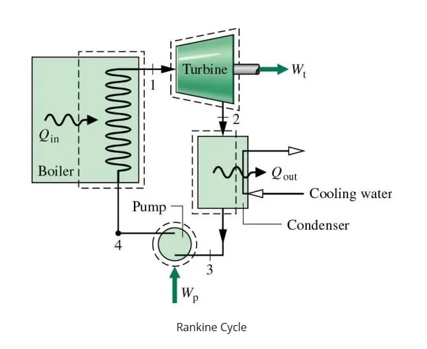
The thermal energy extraction capacity of the Rankin engine varies according to the heat sink temperature and heat source temperature.

According to Carnot’s theorem, the higher the temperature difference, the engine can extract more mechanical energy from thermal energy.

Ideal Rankine Cycle

In the case of the vapour cycle, if the working medium moves over the different parts of a powerplant without any friction pressure and irreversibility loss, the cycle is referred to as the ideal Rankine cycle.

The Rankine cycle is a major working cycle of all power plants in which operating liquid changes continuously from liquid to vapour and vapour to liquid. It is a theoretical cycle in which thermal energy transforms into useful work.

A T-s diagram of the Rankine cycle is given below, which will be helpful to understand the Rankine cycle working.

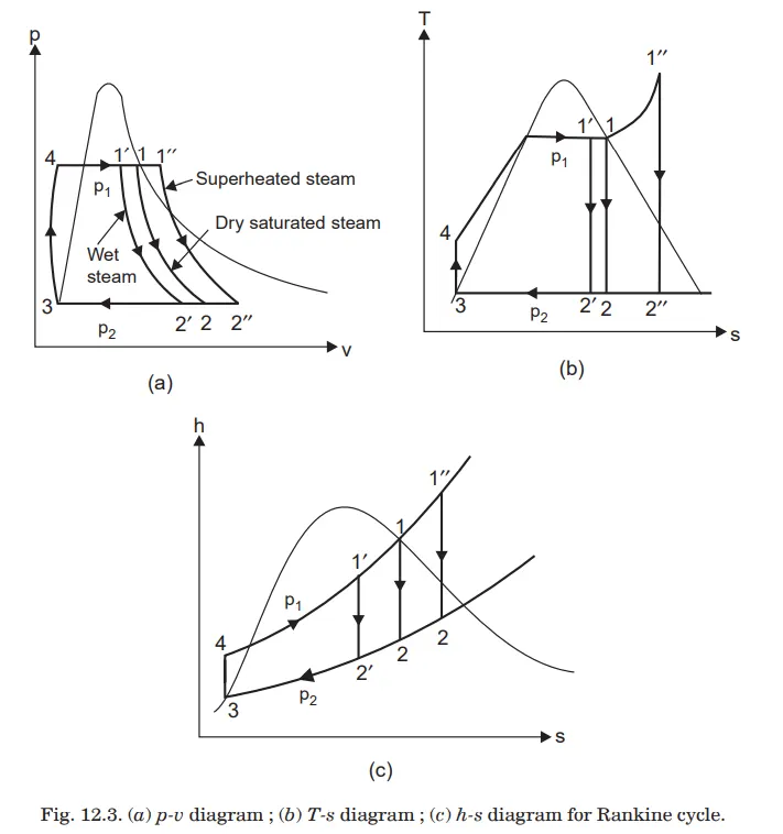
The stages of completing a Rankine cycle are given below:

Isentropic Compression (3 to 4): In this stage, a pump uses to transfer the water or other working medium from the water body (canal or tank etc.) into the boiler. The pump requires a small amount of energy for initial pumping. It pumps the fluid by increasing the pressure of the fluid, but fluid entropy remains the same. For initial pumping, the work done on the pump is given below:
Constant Pressure Heat Addition Process (4 to 1): As the water is delivered into the boiler, an external heat source provides heat to the boiler. The boiler heated the water at constant pressure and converts it into dry saturated vapour (steam). During this process, the enthalpy of the liquid changes, and pressure remains constant.
Isentropic Expansion (1 to 2): After the constant pressure heat addition process, the steam enters into the turbine area, where it expands. As the steam expands, it strikes with the turbine blades, which convert the thermal energy of the steam into rotational energy (mechanical work). As the turbine blades are rotated, they also rotate a crankshaft that further rotates the coil of the generator. As the coil rotates in a magnetic field, it produces electricity. During this whole process, the pressure and temperature of the steam decrease; due to that, some condensation can happen.
Constant Pressure Heat Rejection Process (2 to 3): The vapour or steam enters the condensate tank after the expansion process. In this condensation process, the vapour is condensed to convert it into saturated liquid. During this process, the vapour rejects heat, but its liquid pressure remains the same.

In an ideal Rankine cycle, the turbine and pump work under isentropic conditions. It means the turbine and pump don’t generate entropy; they just increase the performance of the cycle.

The Rankine cycle (shown in the above diagram) avoids the working medium to end up in the superheated vapour area after expanding in the turbine, which decreases the energy dissipated by the condenser.

Actual Rankine Cycle (non-ideal)

In an actual Rankine cycle (or practical power plant), the expansion process in the turbine and compression process in the pump can’t happen under isentropic conditions. In simple words, these are non-reversible processes, and fluid’s internal energy (entropy) increases during these processes.

This cycle raises the required power by the pump to some extent and decreases the turbine’s produced output power.

The formation of water droplets controls the efficiency of steam turbines. When the water droplets condense, they strike the blades of the turbine at high speed; due to that, erosion and pitting occur on the turbine blades. This erosion and pitting gradually reduce the life and productivity of the turbine blades. The simplest method to solve this issue is to superheat the steam.

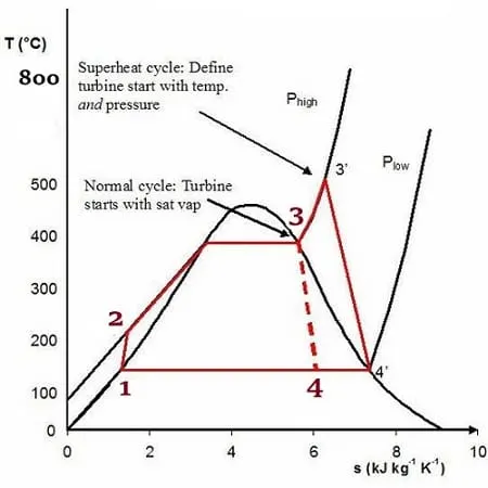
In the above given T-s diagram of the Rankine cycle, state 3 is at the boundary of the two-phase range of water and steam. After expanding, the steam will convert into a very wet form. When steam is superheated, state 3 moves to the right (and up) in the above figure and generates dry steam after expansion.

In modern nuclear power plants the overall thermal efficiency is about one-third (33%), so 3000 MWth of thermal power from the fission reaction is needed to generate 1000 MWe of electrical power. Higher efficiencies can be attained by increasing the temperature of the steam.

Rankine Cycle Equations or Formula

Applying steady flow energy equation (S.F.E.E.) to boiler, turbine, condenser and pump :

(i) For boiler(Process 4 -1) (as control volume), we get
hf4 + Q1 = h1
∴ Q1 = h1 – hf4 ...

(ii) For turbine (Process 1-2)(as control volume), we get
h1 = WT + h2, where WT = turbine work
∴ WT = h1 – h2

(iii) For condenser (Process 2-3), we get
h2 = Q2 + hf3
∴ Q2 = h2 – hf3

(iv) For the feed pump (Process 3-4), we get
hf3 + WP = hf4 , where, WP = Pump work
∴ WP = hf4 – hf3

Now, efficiency of Rankine cycle is given by

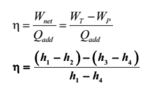
_{Back Work Ratio=WPump/WTurbine=Wp/WT}

_{XSteam Function in MATLAB}

Steam and water properties for Matlab based on the "International Association for Properties of Water and Steam Industrial Formulation 1997 (IAPWS IF-97). A full implementation of the IF-97 standard that provides very accurate steam and water properties in ranges from 0-1000 bar and 0-2000°C. Provided thermodynamic properties are:

Temperature
Pressure
Enthalpy
Specific volume
Density
Specific entropy
Specific internal energy
Specific isobaric heat capacity
Specific isochoric heat capacity
Speed of sound
Viscosity
Vapour fraction

All properties can be calculated with the inputs, p and T known, p and h known, h and s known and some with pressure and density known. X Steam are a full implementation of the IF-97 formulation including all regions and all backward functions for good calculation speed. The code are speed optimized with pressure and enthalpy as inputs for dynamic simulations.

Examples:
XSteam('h_pt',1,20) return the enthalpy of water at 1 bar and 20 degC. 84.0118 kJ/kg

XSteam('rho_ph',1,3000) return the density of steam at 1 bar and 3000 kJ/kg. 0.4056 kg/m3

XSteam('w_pt',1,20) returns the speed of sound at 1 bar and 20 deg C. 1483.4 m/s

XSteam('tSat_p',1) returns the saturation temperature at 1 bar. 99.6059 deg C

The X Steam Tables are the perfect tool both for replacing paper tables and for advanced calculations.

Creat code for calculate cycle parameters

%%%     Rankine cycle   %%%
close all
clear all
clc
disp('              ## Rankine Cycle Simullator ##                 ')

disp('                                                  ')
disp('                                                  ')
disp('     Process  1 - 2 Isentropic Expansion in Condenssor ')
disp('     Process  2 - 3 Constant Pressure Heat Rejection   ')
disp('     Process  3 - 4 Isentropic Compression             ')
disp('     Process  4 - 1 Constant Pressure Heat Addition in Boiler')
disp('                                                  ')


P1=input('Enter the pressure at Turbine Inlate (in bar)=');
T1=input('Enter the Temperature at the Turbine inlet (In Degree celcius)=');
P2=input('Enter the Pressure at the Inlet to Condensor(In bar)=');
disp(' ')

%% Finding the state points parameters of Rankine cycle(1-2-3-4)

%state point 1 turbine inlet 

H1=XSteam('h_pT',P1,T1);
S1=XSteam('s_pT',P1,T1);
Hf1=XSteam('hL_p',P1);    % Saturated liquid enthalpy
Hg1=XSteam('hV_p',P1);    % Saturated vapour enthalpy
Sf1=XSteam('sL_p',P1);    % Saturated Liquid entropy
Sg1=XSteam('sV_p',P1);    % Saturated vapour entropy
Tsat1=XSteam('Tsat_p',P1); %Saturation temperature

disp('       ');

% state point 2 condensor inlet
S2=S1; % isentropic process
Sg2=XSteam('sV_p',P2);     %Saturated vapour entropy
Sf2=XSteam('sL_p',P2);     %Saturated liquid entropy
%S=Sf+xSfg...........we know the equ. of Dryness Fraction
%x=dryness fraction
%Sfg=Sg-Sf
x=(S2-Sf2)/(Sg2-Sf2) ;   %dryness fraction
Hf2=XSteam('hL_p',P2);   %Saturated liquid enthalpy
Hg2=XSteam('hV_p',P2);   %Saturated vapour enthalpy
H2=Hf2+(x*(Hg2-Hf2));
Tsat2=XSteam('Tsat_p',P2);  %Saturation temperature
T2=XSteam('T_hs',H2,S2);    %Temperture as a function of pressure and entropy

disp('          ');

%State point 3
P3=P2;
T3=T2;
H3=Hf2;
S3=Sf2;
disp('     ');

%state point 4
P4=P1;% pump presurre is equal to the inlet pressure at turbine
S4=S3;% steam is compressed isentropicaly  
T4=XSteam('T_ps',P4,S4);%Temperture as a function of pressure and entropy
H4=XSteam('h_ps',P4,S4);%Entalpy as a function of pressure and entropy

disp('     ');

%% Calculating performance characteristics of Cycle %%

%Calculating Turbine work

W_T=H1-H2;

%Calculate Pump Work
W_P=H4-H3;

%Heat supply to Boiler
Q1=H1-H4;

%Net Work done
W_net=(W_T-W_P);

%Thermal Efficiency
Eff=W_net/Q1*100;

%Back work ratio
BWR=W_P/W_T;

%Specific Steam conductivity
SSC=3600/W_T;

%Print the Results in command window
disp('                  RESULTS               ')
%Cycle State point characteristics
fprintf('                At State point 1           \n\n  ')

fprintf('   P1 : %0.3f Bar \n',P1);
fprintf('     T1 : %0.3f Degree celcius \n',T1);
fprintf('     H1 : %3.4f kJ/kg \n',H1);
fprintf('     S1 : %3.4f kJ/kgK \n \n',S1);

  
fprintf('                 At State point 2           \n\n  ')

fprintf('   P2 : %2.3f  Bar \n',P2);
fprintf('     T2 : %2.3f Degre celcius \n',T2);
fprintf('     H2 : %2.4f kJ/kg \n',H2);
fprintf('     S2 : %2.4f kJ/kgK \n \n',S2);


fprintf('                 At State point 3           \n\n  ');

fprintf('   P3 : %2.3f  Bar \n',P3);
fprintf('     T3 : %2.3f Degre celcius \n',T3);
fprintf('     H3 : %2.4f kJ/kg \n',H3);
fprintf('     S3 : %2.4f kJ/kgK \n \n',S3);


fprintf('                 At State point 4           \n\n  ');

fprintf('   P4 : %2.3f  Bar \n',P4);
fprintf('     T4 : %2.3f Degre celcius \n',T4);
fprintf('     H4 : %2.4f kJ/kg \n',H4);
fprintf('     S4 : %2.4f kJ/kgK \n\n',S4);


fprintf('              Cycle Outputs             \n\n ');

fprintf('      Turbine work : %2.4f kJ/kg \n',W_T);
fprintf('      Pump Work : %2.4f kJ/kg \n',W_P);
fprintf('      Net Work : %2.4f kJ/kg \n',W_net);
fprintf('      Thermal Efficiency : %2.4f \n',Eff);
fprintf('      Back Work Ratio : %2.4f \n',BWR);
fprintf('      Specific steam coductivity :%2.4f kg/kWh \n\n',SSC);

%%ploting T-S and H-S Diagram

%ploting saturation curve in T-S Diagram
t=linspace(0,400,600);%split the temperature range in 600 fraction for smooth curve
figure(1)
hold on
for i=1:length(t)        % for loop is used to plot every points
  plot(XSteam('sL_T',t(i)),t(i),'g.');
  plot(XSteam('sV_T',t(i)),t(i),'g.');

end

%plot T-S curve in same figure window
plot([S1 S2],[T1 T2],'color','k','linewidth',2);%plot the 1st,2nd&3rd points of entropy with temperature respectively
plot([S2 S3],[T2 T3],'color','k','linewidth',2);
plot([S3 S4],[T3 T4],'color','k','linewidth',2);
text(S1,T1,'1','fontsize',20);
text(S2,T2,'2','fontsize',20);
text(S3,T3,'3','fontsize',20);

n=linspace(T2,T1,600);
for i=1:length(n)
  plot(XSteam('s_pT',P1,n(i)),n(i),'linewidth',2,'color','k');
  end
plot([Sf1 Sg1],[Tsat1 Tsat1],'linewidth',2,'color','k');
text(Sf1,Tsat1,'4','fontsize',20)
xlabel('Entropy (kJ/kgK)');
ylabel('Temperature (K)');
title('T-S Diagram');
hold off

%plot H-S Diagram
figure(2)
hold on
ts=linspace(0,400,600); %temperature value is to be splited in 600 fraction values
for i=1:length(ts)
  plot(XSteam('sL_T',ts(i)),XSteam('hL_T',ts(i)),'.','color','g');
  plot(XSteam('sV_T',ts(i)),XSteam('hV_T',ts(i)),'.','color','g');
  end
plot([S1 S2 S3 S4 S1],[H1 H2 H3 H4 H1],'color','r','linewidth',2);
xlabel('Entropy (kJ/kgK)');
ylabel('Enthalpy (kJ/kg)');
title('H-S Diagram');
text(S1,H1,'1','fontsize',20);
text(S2,H2,'2','fontsize',20);
text(S3,H3,'3','fontsize',20);
text(S4,H4,'4','fontsize',20);

Code Explanation

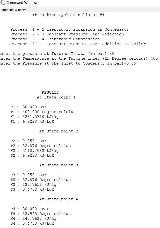
Display the ranckine cycle process 1-2-3-4-1.

Then code write for entering the inputs from user .

Then calculate the various state points in cycle by the use of given XStean file.

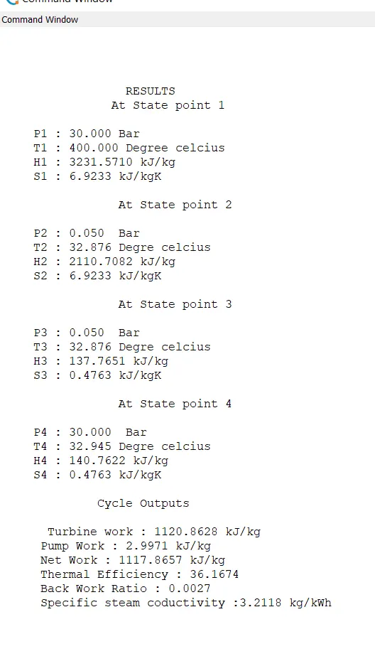
According to thermodynamics formulies we calculate the work done by turbinr,work done bye pump,heat suppy to boiler,heat reliesed in condensor,efficiency of turbine,network done,dryness fraction,specific steam conductivity.

Thes results printed in command window as in below screenshot.

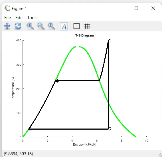
Then plot the saturation curve in T S diagram.

Then plot TS curve in diagram.

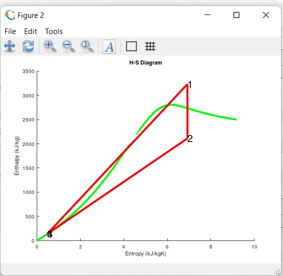
Then we plot the H SDiagram.