Project

AIM:

To carry out a system-level simulation of a BAJA all-terrain vehicle and prepare a technical report explaining the model properties & comments on the results.

OBJECTIVE:

To prepare a technical report on BAJA ATV explaining model properties for the following:

- without using a Lookup table.

- using a Lookup table.

THEORY:

a) ATV:

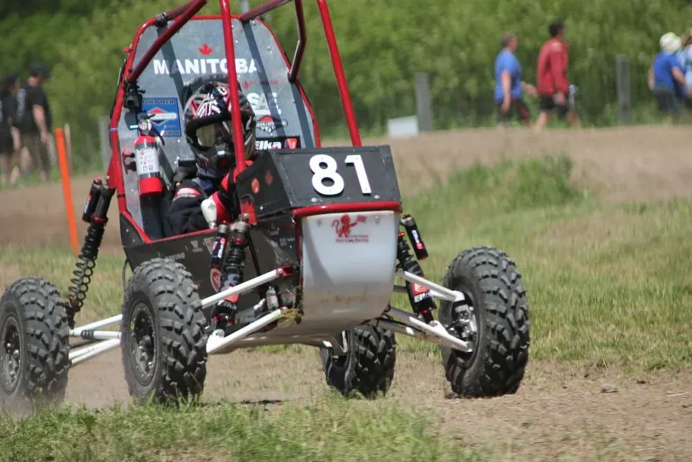
An ATV is an All-terrain vehicle, it is also known as a light utility vehicle (LUV), simply a Quad bike or just a Quad defined by the American National Standards Institute (ANSI). It is a vehicle that travels on low-pressure tires and with a seat straddled by the operator along with steering control with help of a steering wheel or handlebars. It is designed to handle a wide variety of terrain compared to other utility vehicles. Furthermore, it is generally designed for a single operator, but in some cases, it is designed to carry a passenger with the operator. Generally, ATV vehicles are three-wheeled or four-wheeled, in a few cases, it is also 6 wheeled to provide good balance during low-speed operations. ATV vehicles offer better off-road capabilities.

b) CVT (Continuously variable transmission):

Continuously variable transmission is a type of single-speed automatic gearbox. The CVT gearbox has been used in various different cars, but it is usually found and fitted to small cars. CVT is a relatively simple arrangement of two cone-shaped pulleys, With a V-shaped belt connecting them. One pulley is attached to the engine it is called the primary or driving pulley and the other one is joined to the wheels using a simple gear, and is called the driven or secondary pulley. When the accelerator is pressed, the primary cone is rotating according to the power demanded and another cone adjusts accordingly to maintain the same tension in the belt. Since two cones move independently, in effect CVT is a single-speed unit with infinite gear ratios available. When the radius of the primary pulley is greater than the Secondary pulley it is working under overdrive conditions and in conditions where the secondary pulley radius is greater than the primary pulley, it is working under reduced speed.

PROCEDURE:

a. ATV BAJA vehicle model without Look-up table:

1. System-level simulation without dashboard:

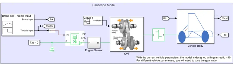
The commonly used blocks in the model:

1. Signal Builder:

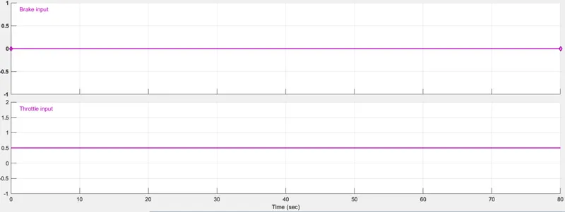
The Signal Builder block allows you to create interchangeable groups of piecewise linear signal sources and use them in a model. It quickly switches the signal groups into and out of a model to facilitate testing. The above model consists of two signals in the signal builder block, one is the throttle signal (0.5) and another is the brake input signal (0), they are kept constant throughout the Simulation.

2. Generic Engine:

The block represents a system-level model of an internal combustion engine. Optional idle speed and red line controllers are included. The block can take throttle or throttle commands as input. The throttle input signal lies between zero and one. Connections F and B are mechanical rotational conserving ports associated with the engine crankshaft and engine block, respectively. Connections P and FC are physical signal output ports through which engine power and fuel consumption rate are reported.

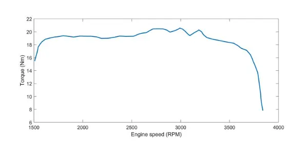
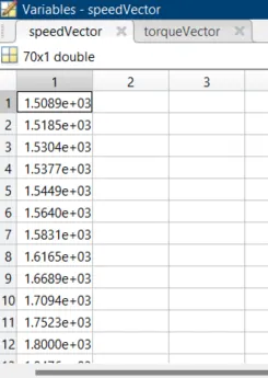
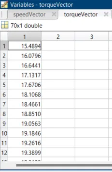
The Speed vector and Torque vector values are assigned in the engine specifications according to the speed torque curve of the BAJA Engine using GRABIT command (Processing data points from the image):

3. Engine sensor Block:

Ideal Rotational motion sensor: The block represents an ideal mechanical rotational motion sensor, that is, a device that converts an across variable measured between two mechanical rotational nodes into a control signal proportional to angular velocity or angle. The sensor is ideal since it does not account for inertia, friction, delays, energy consumption, and so on.

Connections R and C are mechanical rotational conserving ports and connections W and A are physical output ports for velocity and angular displacement, respectively. Only the angular velocity of the engine crankshaft is viewed using a scope, and the angular displacement is terminated using the PS-terminator.

4. Simple Gear:

Here we need to multiply the torque and thus the Simple gear with gear ratio 4 is used. It is a fixed-ratio gearbox. No inertia or compliance is modeled in this block. Connections B (base) and F (follower) are mechanical rotational conserving ports, the relation between B and F rotation directions is specified using the shaft parameters.

5. CVT (Continuously variable transmission):

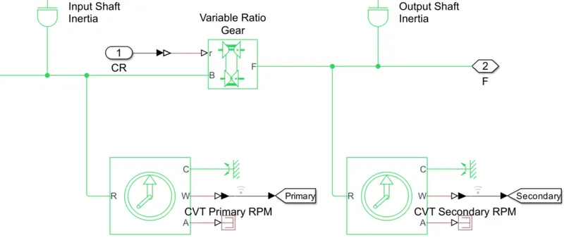
CVT is a subsystem consisting of 2 inertia blocks representing the pulleys and a variable ratio transmission gearbox between them. The angular velocities of the primary (pulley 1) and secondary (pulley 2) shafts are measured using mechanical rotational sensor blocks.

The signal builder block of data points is specified in the cvtratio.mat file provides the gear ratio to the variable gearbox.

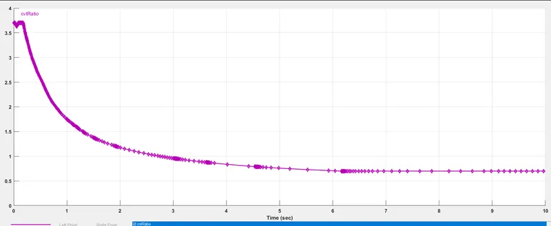
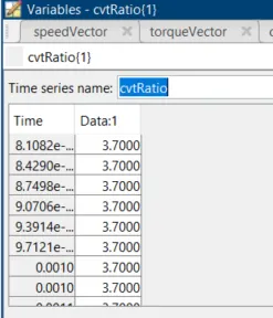
A gear ratio must be ensured before transferring speed to the vehicle body bock. For different vehicle parameters, we can tune the gear ratio.

6. Vehicle Body:

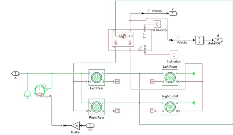
The above image represents a two-axle vehicle body in longitudinal motion. The block accounts for body mass, aerodynamic drag, road incline, and weight distribution between axles due to acceleration and road profile. The vehicle can have the same or a different number of wheels on each axle. Optionally include pitch and suspension dynamics or additional variable mass and inertia. The vehicle does not move vertically relative to the ground.

Connection H is the mechanical translational conserving port associated with the horizontal motion of the vehicle body. The resulting traction motion developed by tires should be connected to this port. Connections V, NF, and NR are physical signal output ports for vehicle velocity and front and rear normal wheel forces, respectively. Wheel forces are considered positive if acting downwards. Connections W and beta are physical signal input ports corresponding to headwind speed and road inclination angle, respectively. If the variable mass is modeled, the physical signal input ports CG and M are exposed. CG accepts a two-element vector representing the x and y distance offsets from vehicle CG to additional load mass CG. M represents the additional mass. If both variable mass and pitch dynamics are included, the physical signal port J accepts the inertia of the additional mass about its own CG.

OUTPUT:

Engine Rpm:

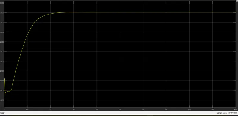
With a constant 0.5 throttle input and zero brake input, the velocity gradually increases to a certain point and then remains the same.

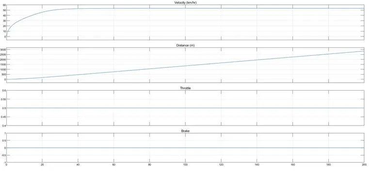
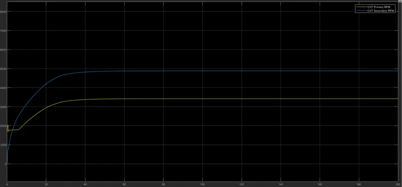
CVT Shaft Speed:

With a fluctuating engine RPM, the CVT maintains smooth transmission and the secondary RPM gradually increases and then remains the same.

2. System-level Simulation with dashboard:

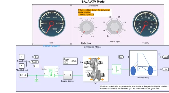
The dashboard has 2 knob throttle inputs and brake input and 2 circular gauges indicating vehicle speed and rpm. This model is similar to the previous model, the only difference being that we can provide throttle input and brake input using the knobs while the simulation is Running.

1. Dashboard: A dashboard (also called dash, instrument panel (IP), or fascia) is a control panel usually located directly ahead of a vehicle's driver, displaying instrumentation and controls for the vehicle's operation.

The initial conditions are as follows:

Brake Input = 0

Throttle Input = 0.5

OUTPUTS:

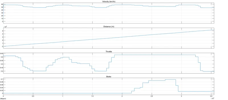
Here below we can observe the throttle demand and the brake input is given by the User by knobs in the dashboard.

We can compare the velocity of the vehicle at the instances where the throttle demand is high and low, also where the brakes are applied the velocity reduces.

CVT Shaft Output:

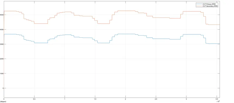
As we can see below, the secondary shaft tries to match the out velocity based on the gear ratio given. Since the input rpm of the ATV engine is limited to 3800 rpm, the out shaft tries to increase close to 5300 rpm depending on the gear ratio given.

b. ATV BAJA vehicle model with Look-up table:

1. System-level simulation without dashboard:

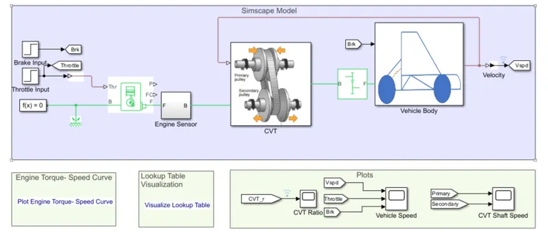
In the model above for BAJA ATV model, including the Look-up table, The CVT ratio to the CVT gearbox is input variably according to the velocity of the vehicle.

Lookup Table: It is an array of data that maps input values to output values, thereby approximating a mathematical function. Given a set of input values, a lookup operation retrieves the corresponding output values from the table. If the lookup table does not explicitly define the input values, Simulink can estimate an output value using interpolation, extrapolation, or rounding, where:

- Interpolation is a process for estimating values that lie between known data points.

A lookup table block uses an array of data to map input values to output values, approximating a mathematical function. Given input values, Simulink performs a “lookup” operation to retrieve the corresponding output values from the table. If the lookup table does not define the input values, the block estimates the output values based on nearby table values.

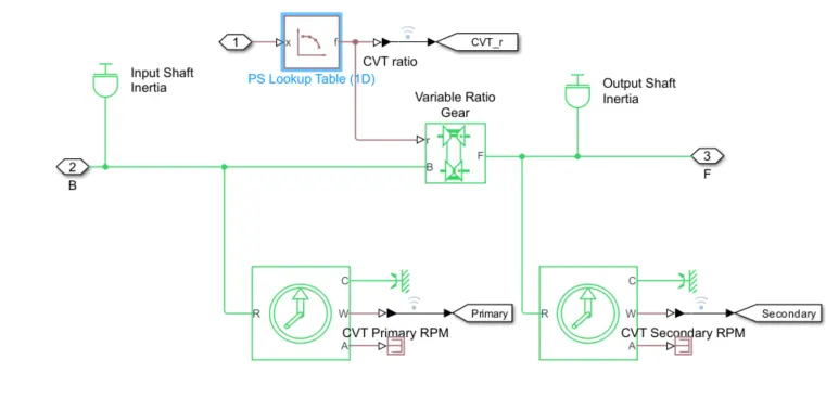
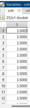
Look-up table representation: CVTR Vehicle speed

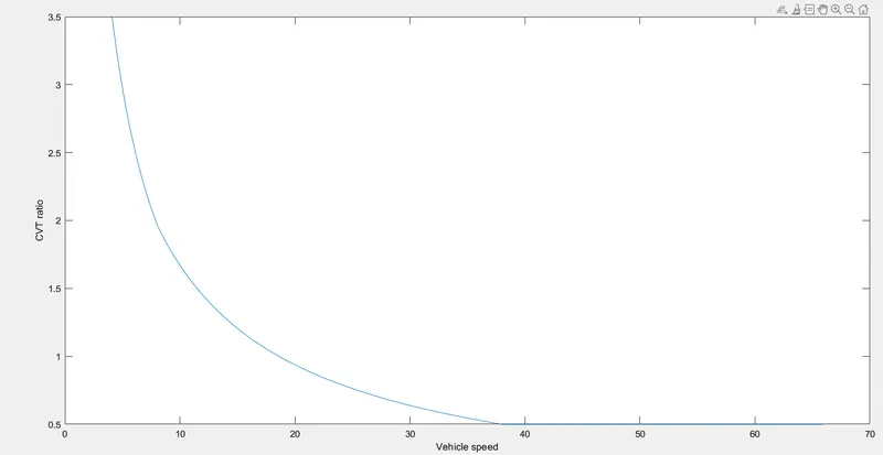
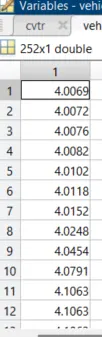
As we can see above, the CVT ratio decreases with an increase in speed. A higher gear ratio provides faster acceleration and a lower gear ratio provides higher top speed.

Throttle and brake inputs:

In this model, the throttle inputs and the brake inputs are given using the step function and not using signal builder signals.

Brake Input: Step time: 35 Initial value: 0 Final value: 0 Sample time: 0

Throttle Input: Step time: 20 Initial value: 0.3 Final value: 1 Sample time: 0

Outputs:

Throttle, brake, and Vehicle speed:

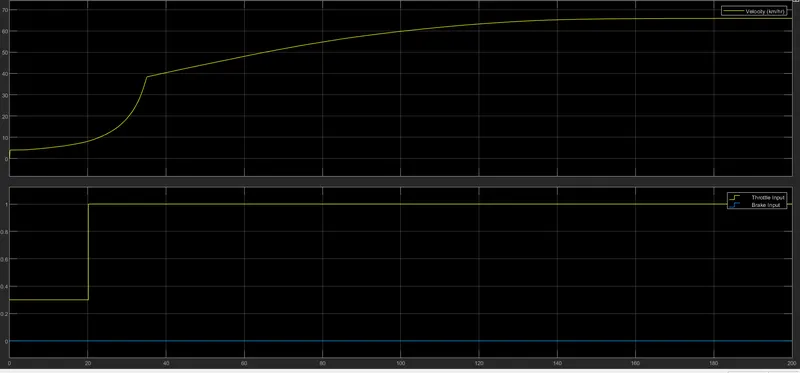
As we can see in the plots, the vehicle accelerates when the torque steps up from 0.3 to 1 at the 20s. Then for the rest of the simulation, the vehicle speed increases gradually.

CVT Shaft speed:

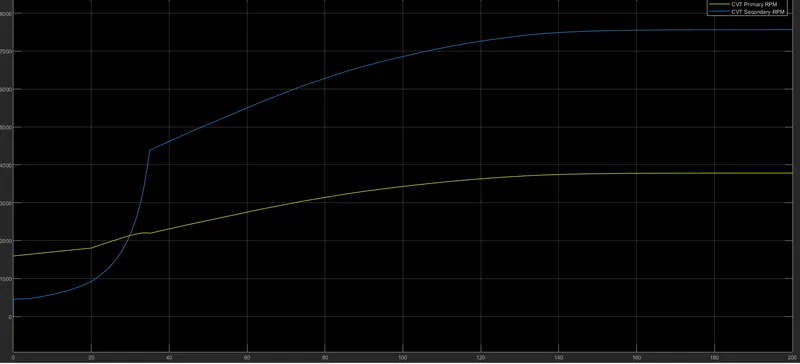
As we can see in the graph, the secondary pulley of the CVT gearbox tries to match the output velocity at the wheels irrespective of the primary shaft. Thus in CVT primary pulley and Secondary pulleys works independently.

CVT ratio output depending on the velocity:

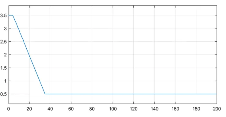
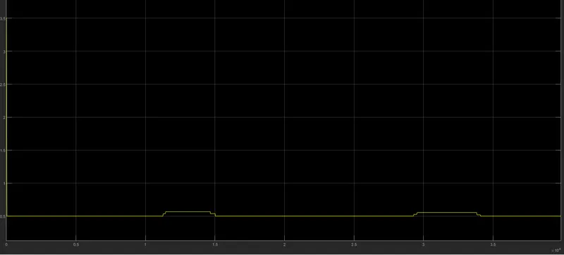
As we can see above, the CVT ratio decreases with an increase in speed. A higher gear ratio provides faster acceleration and a lower gear ratio provides higher top speed.

2. System-level Simulation with Dashboard:

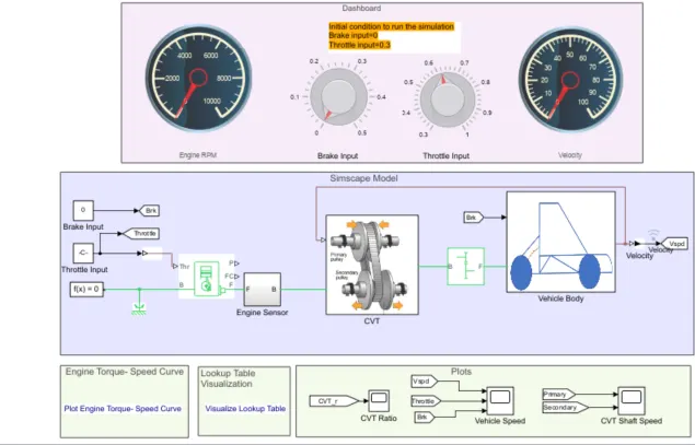
The above model is similar to the previous model the only difference is the throttle input and the brake input is given with help of the Knobs in the dashboard. The CVT ratio is given to the Cgearboxboc by the Lookup table, Lookup table maps the input velocity values to the output values of the CVT ratio.

The Model simulation is run for an infinite time and the throttle input and brake input is being varied as required by the User and the simulation is manually stopped after a certain interval.

Output:

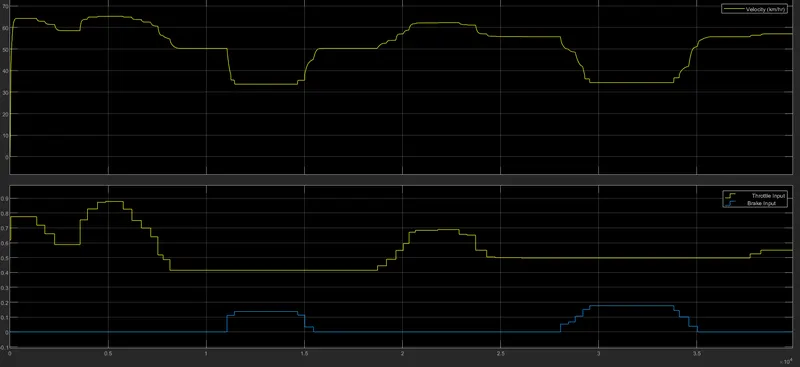
Vehicle speed Output:

As we can see the throttle is increased to a higher speed initially and is reduced when the brakes are applied. With inputs of throttle and brakes, the vehicle speed is varied which can be seen in the velocity plot.

CVT ratio Output:

Conclusion:

Hence, the given BAJA ATV Model was simulated successfully and from the above results, we can infer that:

- Velocity, CVT Shaft Speed, and Engine Speed are directly proportional to the Throttle input and inversely proportional to the Brake input.

- CVT Ratio is directly proportional to the Torque and inversely proportional to the Throttle input.

- CVT Primary speed is greater than CVT Secondary speed as they are directly proportional to their shaft diameter.

- All models are fully focused on CVT, and this project will be able to show the effect of CVT on the vehicle behavior of different models of ATVs.

References:

https://in.mathworks.com/matlabcentral/fileexchange/70576-baja-all-terrain-vehicle-atv-model