Project

AIM:

Carry out a system-level simulation of an all-terrain vehicle (Download the model from provided link).

Objective:

Prepare a technical report explaining the model properties & comments on the results.

INTRODUCTION:

About ATV:

ATVs are motorized vehicles that are meant to be used off-road or on dirt roads, not on paved roads or highways. They usually have four large balloon-style tires, with a seat in the middle that a rider straddles while steering by the handlebars. There are still some three-wheeler ATVs around, but manufacturers stopped making them in 1988 due to concerns about stability and safety.

Weighing more than 600 pounds, ATVs have large, powerful engines that allow them to reach speeds of 65 mph or more. They have a high center of gravity and no roll bars, safety cages, or seatbelts, meaning they can tip easily, throw riders and passengers off, or even roll over on top of riders. This can cause serious injury or death, usually because of head injuries. Other common injuries include cuts, scrapes, broken collarbones, and broken arms and legs.

About CVT:

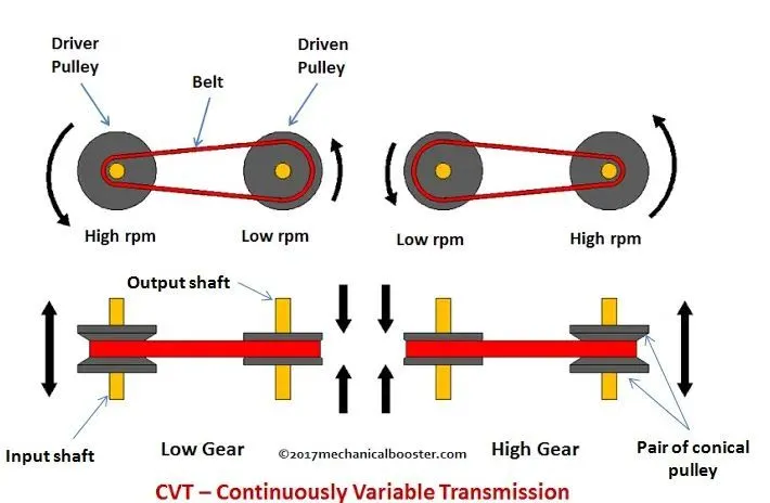
The most common type of CVT uses a V-belt which runs between two variable-diameter pulleys. The pulleys consist of two cone-shaped halves that move together and apart. The V-belt runs between these two halves, so the effective diameter of the pulley is dependent on the distance between the two halves of the pulley. The V-shaped cross-section of the belt causes it to ride higher on one pulley and lower on the other; therefore, the gear ratio is adjusted by moving the two sheaves of one pulley closer together and the two sheaves of the other pulley farther apart.

As the distance between the pulleys and the length of the belt does not change, both pulleys must be adjusted (one bigger, the other smaller) simultaneously in order to maintain the proper amount of tension on the belt. Simple CVTs combining a centrifugal drive pulley with a spring-loaded driven pulley often use belt tension to affect the conforming adjustments in the driven pulley. The V-belt needs to be very stiff in the pulley's axial direction in order to make only short radial movements while sliding in and out of the pulleys.

The radial thickness of the belt is a compromise between the maximum gear ratio and torque. Steel-reinforced V-belts are sufficient for low-mass, low-torque applications like utility vehicles and snowmobiles, but higher-mass and -torque applications such as automobiles require a chain. Each element of the chain must have conical sides that fit the pulley when the belt is running on the outermost radius. As the chain moves into the pulleys the contact area gets smaller. As the contact area is proportional to the number of elements, chain belts require many very small elements.

About Baja SAE:

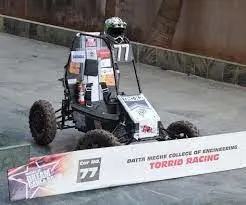
Baja SAE consists of competitions that simulate real-world engineering design projects and their related challenges. Engineering students are tasked to design and build an off-road vehicle that will survive the severe punishment of rough terrain. Each team's goal is to design and build a single-seat, all-terrain, sporting vehicle whose structure contains the driver. The vehicle is to be a prototype for a reliable, maintainable, ergonomic, and economic production vehicle which serves a recreational user market.

SIMPLE CVT MODEL:

File contained includes BAJA ATV model with Continuously Variable Transmission (CVT). These models show how to build an ATV with CVT which is mostly used in BAJA competitions. Simscape and Simscape Driveline have been used to complete the system. The engine data used in the model is provided as an image which shows the Engine Speed (RPM) Vs Torque curve. This is an open loop model of CVT.

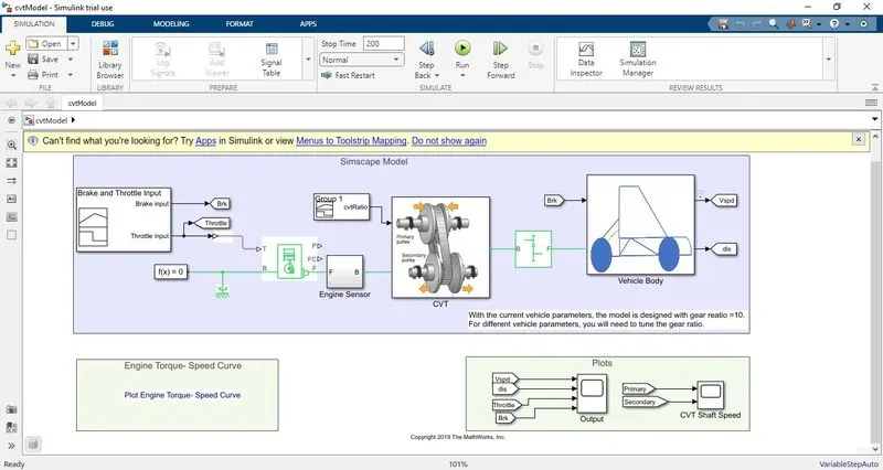
We can see in the above model the input for engine is acceleration (Throttle). Then the engine was connected with CVT and gave rpm input to CVT. The secondary pulley of CVT gave input to simple gear and then simple gear input to vehicle body block in vehicle body subsystem. all output from system is given to output with the help of Goto and from block. Input for engine, CVT and vehicle body from the signal builder block.

In the above model ATV model was made with some inbuild blocks and subsystems as follows,

GENERIC ENGINE

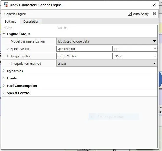
Generic engine block is a system-level model of spark-ignition and diesel engines suitable for use at initial stages of modeling when only the basic parameters are available. Optional idle speed and red line controllers are included. The throttle input signal T lies between zero and one and specifies the torque demanded from the engine as a fraction of the maximum possible torque. If the engine speed falls below the Stall speed, the engine torque is blended to zero. If the engine speed exceeds the Maximum speed, the simulation stops and issues an error message. Connections F and B are mechanical rotational conserving ports associated with the engine crankshaft and engine block, respectively. Connections P and FC are physical signal output ports through which engine power and fuel consumption rate are reported.

PARAMETERS:

INPUT FOR ENGINE:

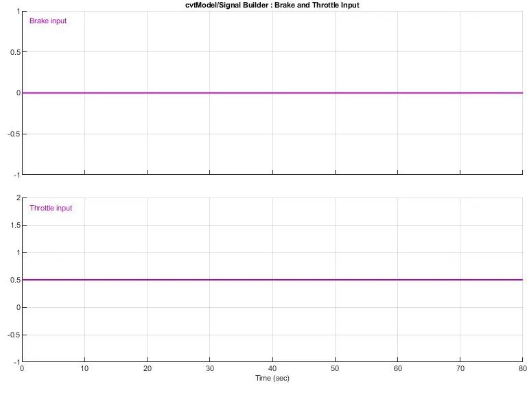
Signal builder is used to give two inputs. Throttle and breaking these are two inputs for engine.

We can observe that currently there is no break input and a constant throttle is provided to the system. Here the data for engine speed and torque is extracted from the following image of speed and torque data with the help of GRABIT file exchange option. This function extracts the data point from image and saved in workspace to use.

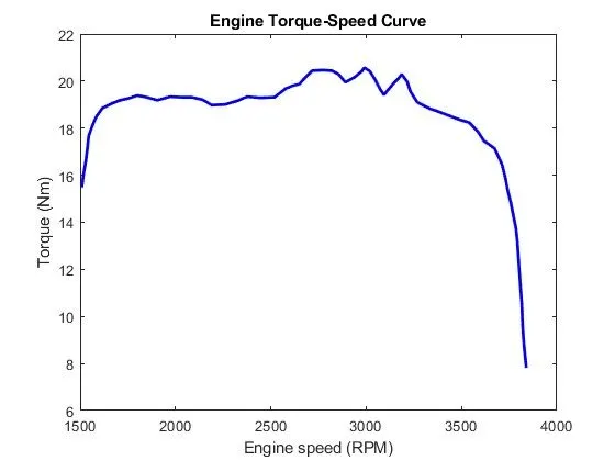
GRABIT information source: - File Exchange – GRABIT

ENGINE RPM AND SENSOR

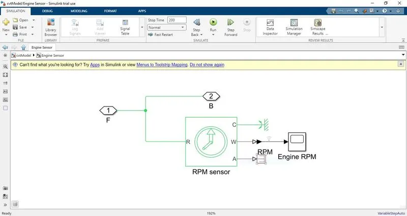
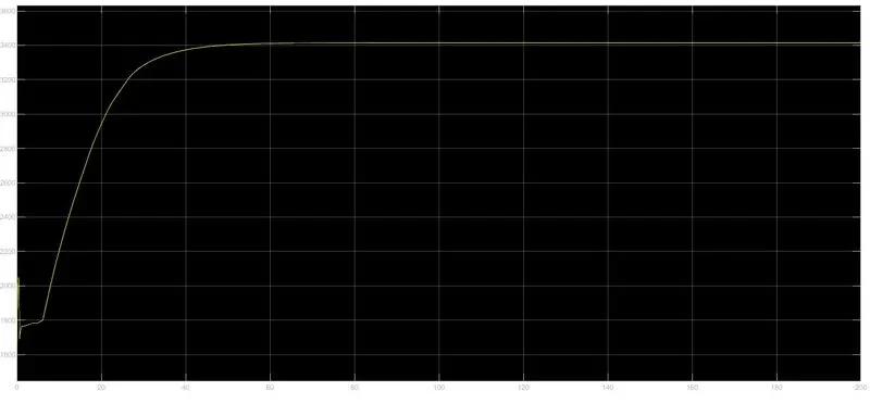
Engine sensor is the Ideal Rotational Motion Sensor block represents an ideal mechanical rotational motion sensor, that is, a device that converts an across variable measured between two mechanical rotational nodes into a control signal proportional to angular velocity or angle. You can specify the initial angular position (offset) as a block parameter. The sensor is ideal since it does not account for inertia, friction, delays, energy consumption, and so on. Connections R and C are mechanical rotational conserving ports that connect the block to the nodes whose motion is being monitored. Connections W and A are physical signal output ports for velocity and angular displacement, respectively.

CVT TRANSMISSION:

1. Go to: - Send signals to from blocks that have the specified tag. If tag visibility is 'scoped', then a Goto Tag Visibility block must be used to define the visibility of the tag. The block icon displays the selected tag name (local tags are enclosed in brackets, [], and scoped tag names are enclosed in braces, {}).
2. Inport: - Provide an input port for a subsystem or model.
3. Inertia: - The block represents an ideal mechanical rotational inertia.
4. PMC_port: - Physical Modelling Connection Port block for subsystems.
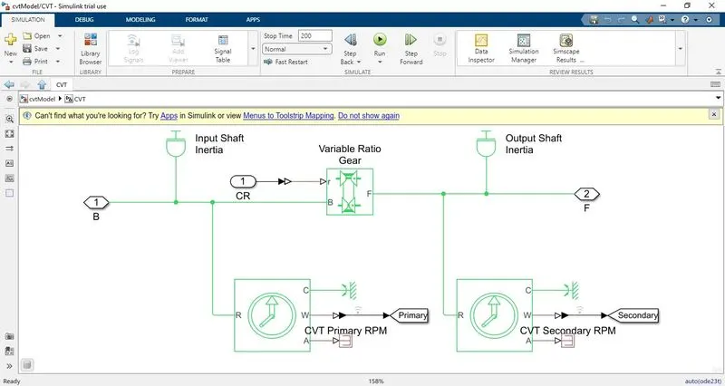
5. Variable ratio gear transmission: - Represents a variable ratio gearbox such as implemented by mechanical belt CVT, electric, or hydraulic transmissions. The physical signal input r defines the ratio of input to output angular shaft velocities. Connections B (base) and F (follower) are mechanical rotational conserving ports. Specify the relation between base and follower rotation directions with the Output shaft rotates parameter.
6. Ps terminator: - Use this block to terminate physical signal outputs. Unconnected physical signal output ports do not generate warnings, but connection to a PS Terminator can be used to indicate that the signal was not inadvertently left unconnected.
7. Mechanical Rotational Reference: - This block represents a mechanical rotational reference point, that is, a frame or a ground. Use it to connect mechanical rotational ports that are rigidly affixed to the frame (ground).
8. PS-Simulink Converter: - Converts the input Physical Signal to a Simulink output signal.
9. The unit expression in 'Output signal unit' parameter must match or be commensurate with the unit of the Physical Signal and determines the conversion from the Physical Signal to the Simulink output signal.

CVT SUBSYSTEM:

INPUT FOR CVT:

VEHICLE BODY:

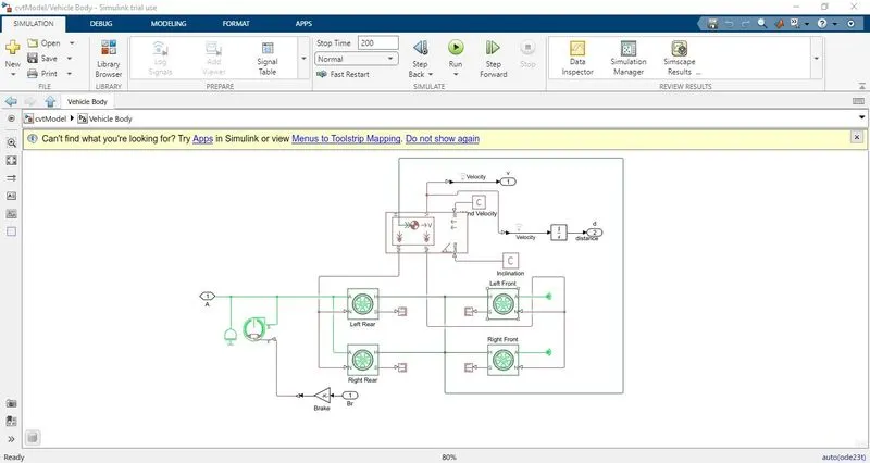
Two axle vehicles with longitudinal dynamics and motion with adjustable mass, geometry and drag properties. The vehicle can have the same or a different number of wheels on each axle. For e.g.; two wheels on the front axle and one wheel on the rear axle. The vehicle wheels are assumed identical in size.

FLOW PROCESS

• The throttle signal is generated by the signal builder block and inputted to the generic engine.
• The torque and speed vector are inputted from the MATLAB workspace.
• The engine will generate the output rpm which we can take from the crank shaft output.
• This is further will be given in to the ideal rotational motion sensor to sense the output rpm.
• The same output speed is given to a simple gear mechanism to reduce the speed where the gear ratio taken is 4.
• The output speed from the gear reducer will be given to the variable ratio Transmission block.
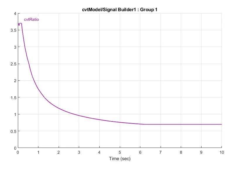
• Using the signal builder, the CVT ratio is given to the respective block.
• The speed is controlled by the variable CVT ratios and the controlled output speed is inputted to the axle.
• The brake signal is generated by the signal builder and inputted to the vehicle body for applying the brake.
• The power from the CVT is inputted to the axle and hence the vehicle get accelerated according to the speed.
• The velocity is taken as the output for further analysis.

OUTPUT RESULTS:

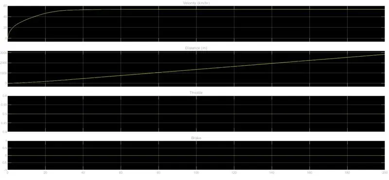
In the above graph we can see that the velocity increases over time to 40 sec but after that it will constant. We cover a 3km distance with 0.5 throttled input and no brake applied.

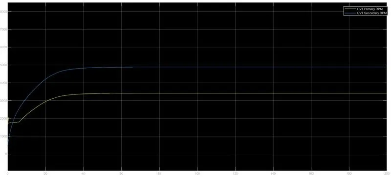
CVT SHAFT SPEED:

Here we can see that the secondary pulley rpm is greater than primary pulley because when we accelerate the vehicle the primary pulley will expand and secondary pulley will extract this process is nothing but speed reduction.

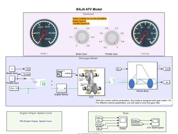
BAJA ATV MODEL WITH DASHBOARD:

FLOW PROCESS

The model work flow process is same as the process of BAJA ATV model without dashboard, but the throttle and brake inputs are controlled by the user with the knob provided. We can change the inputs brake and throttle by changing the knob values provided.

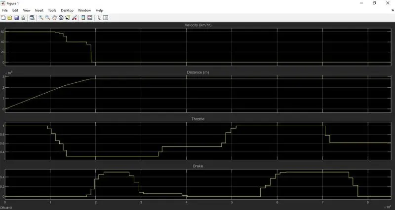
OUTPUT:

Here we can see that the response of model to the throttle input and brake input. When we start the simulation the velocity at 60km/hr then we reduce throttle gradually then velocity also decreased. When we apply a brake then also, we can see that the velocity decreased so we can say that the vehicle speed totally depends on throttle and brake input.

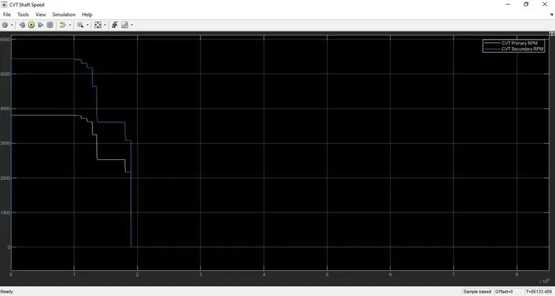
CVT SHAFT SPEED:

MODEL: - (simple CVT Model Data Extraction):

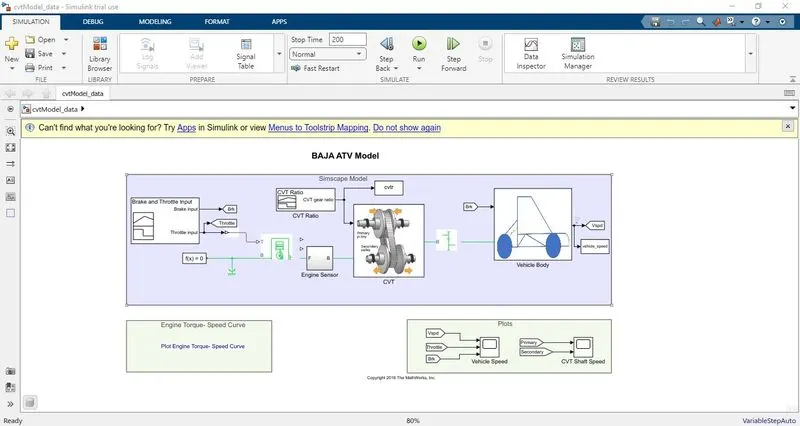
Here we are only changing our input data for more visualization.

New inputs:

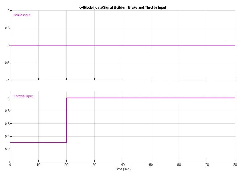
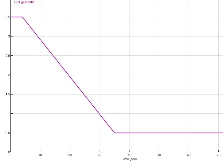
New outputs:

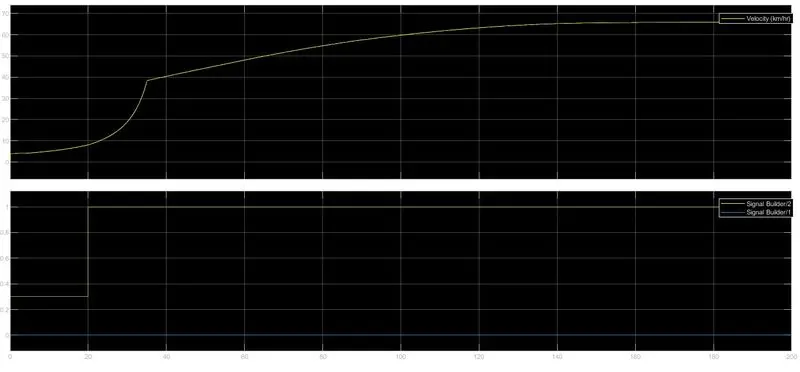
Here we can see that we give input throttle and brake and velocity graph also responding according to input given.

CVT SHAFT SPEED:

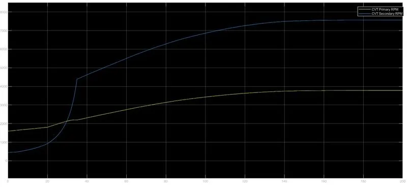
Here we can observe till 30 sec the secondary pulley RPM is less than secondary because input we gave sudden acceleration after 20 second then constant to 1. So, after 30 again the secondary pully rpm increased and primary pully rpm decreased. Hence, we can say that till 30sec the CVT is in overdrive and after 30 sec in speed reduction drive.

Here we used a simple model to extract the CVR ratio data.

Code to extract data:

%% Load and simulate the model
cvtModel_data
sim('cvtModel_data')

%% Visualize the lookup table 
plot(vehicle_speed,cvtr,'r','LineWidth',2)
xlabel ('Vehicle Speed (km/hr)')
ylabel ('CVT Ratio')
title ('Lookup Table Visualization')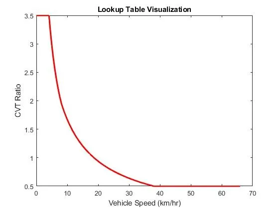

FLOW PROCESS:

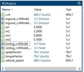
The model workflow process is same as the process of 'BAJA ATV MODEL WITHOUT DASHBOARD' the change here is that the CVT ratio and vehicle speed data are extracting from the base workspace.

WORKSPACE:

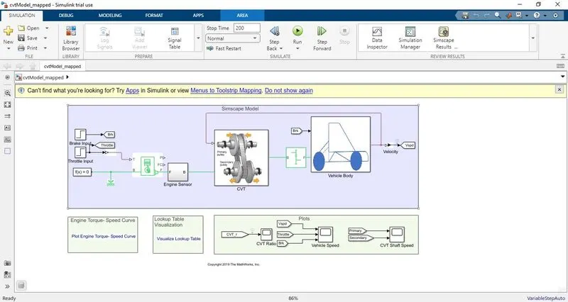
MODEL: - (Mapped CVT Model):

FLOW PROCESS

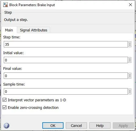
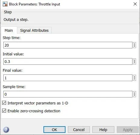
Instead of signal builder blocks for brake and throttle inputs, the step blocks are used. At 35 sec the brake input will take a step value of 0 and at 20 sec throttle input will increase from 0.3 to 1 then remains constant throughout. instead of signal builder block for CVT ratio the 2D Look up table is used.

Blocks used in model: -

Lookup table: - A lookup table is an array of data that maps input values to output values, thereby approximating a mathematical function. Given a set of input values, a lookup operation retrieves the corresponding output values from the table. If the lookup table does not explicitly define the input values, Simulink can estimate an output value using interpolation, extrapolation, or rounding, where:

• An interpolation is a process for estimating values that lie between known data points.
• An extrapolation is a process for estimating values that lie beyond the range of known data points.
• A rounding is a process for approximating a value by altering its digits according to a known rule.

A lookup table block uses an array of data to map input values to output values, approximating a mathematical function. Given input values, Simulink performs a “lookup” operation to retrieve the corresponding output values from the table. If the lookup table does not define the input values, the block estimates the output values based on nearby table values.

Since table lookups and simple estimations can be faster than mathematical function evaluations, using lookup table blocks might result in speed gains when simulating a model. Consider using lookup tables in lieu of mathematical function evaluations when:

• An analytical expression is expensive to compute.
• No analytical expression exists, but the relationship has been determined empirically.

INPUT FOR STEP BLOCK:

INPUT FOR CVT RATIO:

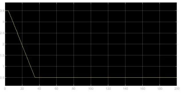
OUTPUT RESULTS:

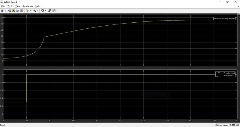
Here we can observe till 40 sec the secondary pulley RPM is less than secondary because input we gave sudden acceleration after 20 second then constant to 1. So, after 40sec again the secondary pully rpm increased and primary pully rpm decreased. Hence, we can say that up to 40sec the CVT is in overdrive and after 40 sec in speed reduction drive.

BAJA ATV MODEL - MAPPED CVT MODEL WITH DASHBOARD

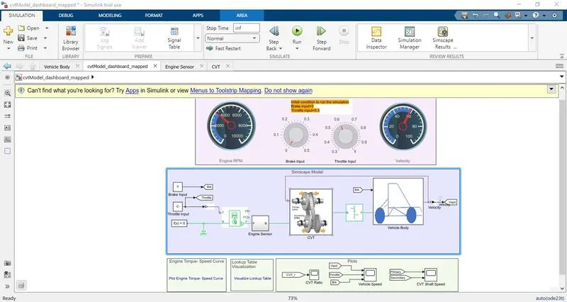
BAJA ATV model mapped lookup table with dashboard is also similar as the process of 'mapped lookup table without dashboard' here the throttle and break inputs are controlled by the knobs provided in the dashboard.

OUTPUT RESULTS:

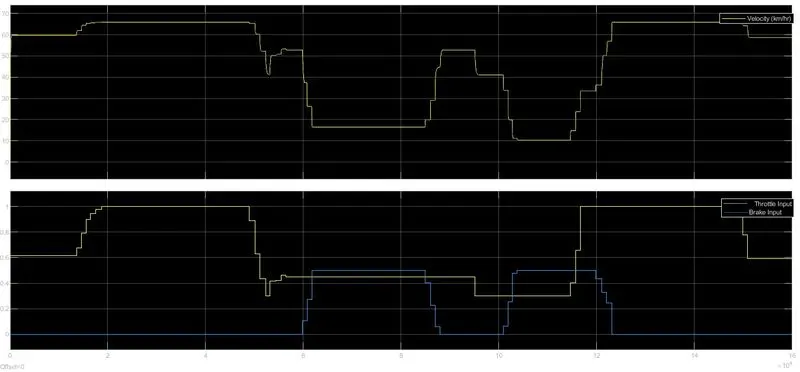
In the above figure we can see that velocity follows the same path as the input which is throttle input and brake input.

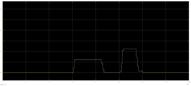
CVT GEAR RATIO:

CVT SHAFT SPEED:

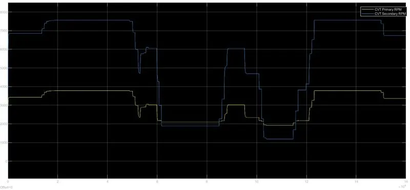
Here we can see that the velocity and CVT RPM graph are identical and primary pulley rpm is less than the secondary pulley rpm because we are using speed reduction drive for CVT.

CONCLUSION:

We can conclude that we have successfully simulated the Baja All-Terrain Vehicle with different methods like open loop model and close loop model. We got satisfactory results for the simulation. We can use this model to simulate actual data for SAE competition.

CLICK HERE TO SEE MODEL AND PHOTO