Week 4.1 - Genetic Algorithm

AIM:

1. Write a code in MATLAB to optimize the stalagmite function and find the global maxima of the function.
2. explain the concept of genetic algorithm and also explain the syntax for ga in MATLAB.
3. Plot graphs for all 3 studies and for F maximum vs no. of iterations.

GOVERNING EQUATIONS:

Objective:

1. To write a code in MATLAB to optimize the stalagmite function and find the global maxima of the function by using ga command.
2. To explain the concept of genetic algorithm and also explain the syntax for ga in MATLAB.
3. To Plot graphs for all 3 studies and for F maximum vs no. of iterations by plot command

Introduction:

+ Genetic algorithm starts with an initial set of random solutions called population.

+ Each individual in the population is called a chromosome representing a solution to the problem at hand.

+ The chromosomes evolve through successive iterations, called generations.

+ During each generation, the chromosomes are evaluated using some measures of fitness.

+ To create the next generation, new chromosome, called offspring, are formed by either (a) merging two chromosomes from current generation using a crossover operator or (b) modifying a chromosome using a mutation operator.

+ A new generation is formed by (a) selecting, according to the fitness values, some of the parents and offspring and (b) rejecting others so as to keep the population size constant.

+ Fitter chromosomes have higher probabilities of being selected.

+ After several generations, the algorithms converge to the best chromosome, which hopefully represents the optimum or suboptimal solution to the problem.

Getting maxima using ga:

Ga is inbuilt function in matlab which gives minimum optimum solution but in our problem we want maximum value for that we uses negative sign while defining the equation.

Syntax for ga:

x = ga(fun,nvars) finds a local unconstrained minimum, x, to the objective function, fun. nvars is the dimension (number of design variables) of fun.

x = ga(fun,nvars,A,b)

x = ga(fun,nvars,A,b,Aeq,beq)

x = ga(fun,nvars,A,b,Aeq,beq,lb,ub) defines a set of lower and upper bounds on the design variables, x, so that a solution is found in the range lb ≤ x ≤ ub. (Set Aeq=[] and beq=[] if no linear equalities exist.)

x = ga(fun,nvars,A,b,Aeq,beq,lb,ub,nonlcon)

x = ga(fun,nvars,A,b,Aeq,beq,lb,ub,nonlcon,options)

x = ga(fun,nvars,A,b,Aeq,beq,lb,ub,nonlcon,intcon)

x = ga(fun,nvars,A,b,Aeq,beq,lb,ub,nonlcon,intcon,options)

Explaination of coading:

1. In below code I use clc, clear all and close all to remove all previous data.
2. Then I use function command to create function given in problem in separate window
3. In main program I define the line space for x and y, also number of iterations
4. After that I use mesh grid command to create 2D array.
5. Then for evaluation I uses the for-loop command.
6. In loop command I uses input vectors for giving inputs to the stalagmite function which is coded in separate window.
7. In case 1 I use only function and number of variables without boundaries of inputs
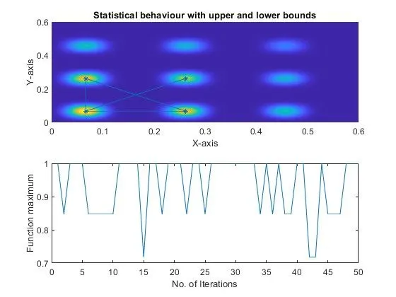
8. In case 2 I use only function and number of variables with boundaries of inputs
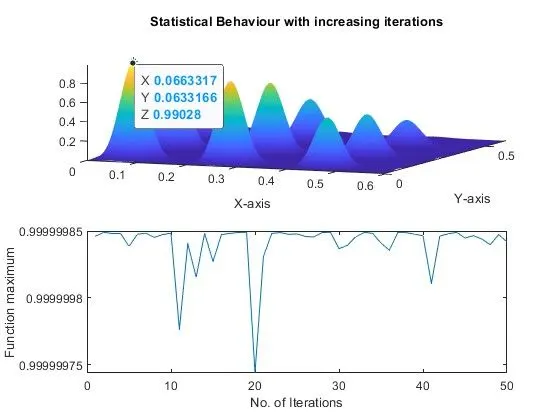
9. In case 3 I uses only function and number of variables with boundaries of inputs and I increases the number of iterations to 400 by using option in ga syntax.

CODE FOR STALAGMITE FUNCTION:

%Define Stalagmite Function

function [f] = stalagmite(input_vector)
x = input_vector(1);
y = input_vector(2);

t1 = (sin((5.1*pi*x)+0.5))^6;
t2 = (sin((5.1*pi*y)+0.5))^6;
t3 = exp(-4*log(2)*((x-0.0667)^2)/0.64);
t4 = exp(-4*log(2)*((y-0.0667)^2)/0.64);

f = -(t1*t2*t3*t4);
end

CODE FOR OPTIMUM SOLUTION:

clear   % To clear previous output
close all % used for close all open windows if any.
clc

%Define our search space
x = linspace(0,0.6,200);         %x array
y = linspace(0,0.6,200);         %y array
n = 50;                          %number of cases

%Creating a 2D mesh
[xx, yy] = meshgrid(x,y);

%Evaluating a stalagmite function
for i = 1:length(xx)
    for j = 1:length(yy)
        input_vector(1)=xx(i,j);
        input_vector(2)=yy(i,j);
        f(i,j) = stalagmite(input_vector);
    end
end

%Study 1 : Statistical Behaviour

tic
for i = 1:n
    [inputs,fopt(i)] = ga(@stalagmite,2);
    xopt(i) = inputs(1);
    yopt(i) = inputs(2);
end

study1_time = toc  % gives time for 1st study

figure(1)
subplot(2,1,1)
hold on
surfc(xx,yy,-f)
shading interp
xlabel('X-axis')
ylabel('Y-axis')
title('Statistical Behaviour with Unbound inputs')
plot3(xopt,yopt,-fopt,'marker','*','markersize',4,'markerfacecolor','b')
subplot(2,1,2)
plot(-fopt)
xlabel('No. of Iterations')
ylabel('Function maximum')

%Study2 : Statistical behaviour with upper and lower bounds

tic
for i = 1:n
    [inputs,fopt(i)] = ga(@stalagmite,2,[],[],[],[],[0;0],[1;1]);
    xopt(i) = inputs(1);
    yopt(i) = inputs(2);
end

study2_time = toc % gives time for 2nd study
figure(2)
subplot(2,1,1)
hold on
surfc(xx,yy,-f)
shading interp
xlabel('X-axis')
ylabel('Y-axis')
title('Statistical behaviour with upper and lower bounds')
plot3(xopt,yopt,-fopt,'marker','*','markersize',4,'markerfacecolor','y')
subplot(2,1,2)
plot(-fopt)
xlabel('No. of Iterations')
ylabel('Function maximum')

%Study3 : Statistical Behaviour with increasing iterations of GA

options = optimoptions('ga');
options = optimoptions(options,'PopulationSize',400);

tic
for i = 1:n
    [inputs,fopt(i)] = ga(@stalagmite,2,[],[],[],[],[0;0],[1;1],[],[],options);
    xopt(i) = inputs(1);
    yopt(i) = inputs(2);
end


study3_time = toc % gives time for 1st study

figure(3)
subplot(2,1,1) % use to create 2 plot in single figure
hold on
surfc(xx,yy,-f)
shading interp
xlabel('X-axis')
ylabel('Y-axis')
title('Statistical Behaviour with increasing iterations')
plot3(xopt,yopt,-fopt,'marker','*','markersize',5,'markerfacecolor','m')
subplot(2,1,2)
plot(-fopt)
xlabel('No. of Iterations')
ylabel('Function maximum')

Results:

In first case I getting different-different results as I have not specified the limits in GA syntax.This problem was solved in second case by giving the boundaries fir inputs variables. But again the optimum value is varies this problem is resolved by increasing number of iteration in third case.

All results and plots for different – different case is shown below.

CASE 1

CASE 2

CASE 3

Conclusion:

I learn the ga command. Find the way for to get maximum optimum value. And also, I learn how to use ga commend with its syntax.