Project

AIM:  

To Study and analyze the BAJA All Terrain Vehicle ATV( All terrain Vehical) model using Simulink by given link (https://www.mathworks.com/matlabcentral/fileexchange/70576-baja-all-terrain-vehicle-atv-model)

OBJECTIVES:

•  To prepare a technical report of Baja ATV model.

 TYPES OF MODEL:

• BAJA ATV model without Dashboard.
• BAJA ATV model with Dashboard.

MAIN MODEL:

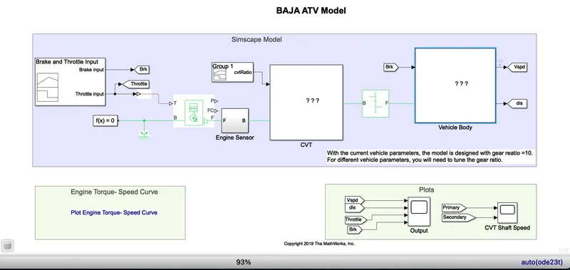
MAJOR COMPONENTS USED IN THIS SIMULATION:

GENERIC ENGINE:

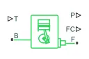
The Generic Engine block represents a general Internal Combustion (IC) Engine, which is a type of Spark Ignition (SI-Petrol) or Compression Ignition (CI-Diesel). The speed torque and speed power parameters are provided.

Ports:

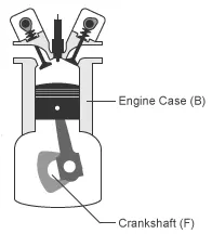
• B – Rotational Conserving Port representing the Engine Block
• F – Rotational Conserving Port representing the Engine Crankshaft
• T – Physical signal input port specifying the normalized engine throttle level
• P – Physical signal output port reporting the instantaneous engine power, in Watts (W)
• FC – Physical signal input port reporting the fuel consumption rate, in kg/s.

ENGINE SENSOR:

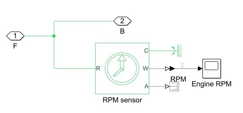
This block measures angular velocity or angle in a mechanical rotational network. The sensor is ideal since it does not account for inertia, friction, delays, energy consumption, and so on.The physical signal ports W and A report the angular velocity and angular displacement, respectively, of port R relative to port C. The measurement is positive when the motion at R is greater than the motion at C.

SIMPLE GEAR:

The simple gear is a combination of a driver and driven gear where the speed is reduced by the gear ratio. The gear ratio is defined as,

 

Ports:

• B – Base Gear or Driver Gear.
• F – Follower Gear or Driver Gear.

CVT (Continuous Variable Transmission) SYSTEM:

In CVT (Continuous Variable Transmission), the variable diameter pulley plays a vital role in transmission. Variable – diameter pulleys must always come in pairs. One of the pulleys, known as the drive pulley (or driving pulley), is connected to the crankshaft of the engine. The driving pulley is also called the input pulley because it’s where the energy from the engine enters the transmission. The second pulley is called the driven pulley because the first pulley is turning it. As an output pulley, the driven pulley transfers energy to the driveshaft.The distance between the center of the pulleys to where the belt makes contact in the groove is known as the pitch radius. When the pulleys are close together, the belt rides higher and the pitch radius increases. The ratio of the pitch radius on the driving pulley to the pitch radius on the driven pulley determines the gear when the pitch radius is small on the driving pulley and large on the driven pulley, then the rotational speed of the driven pulley decreases, resulting in a lower “gear”. When the pitch radius is large on the driving pulley and small on the driven pulley, then the rotational speed of the driven pulley increases, resulting in a higher “gear”. Thus, in theory, a CVT has an infinite number of “gears” that it can run through at any time, at any engine or vehicle speed.

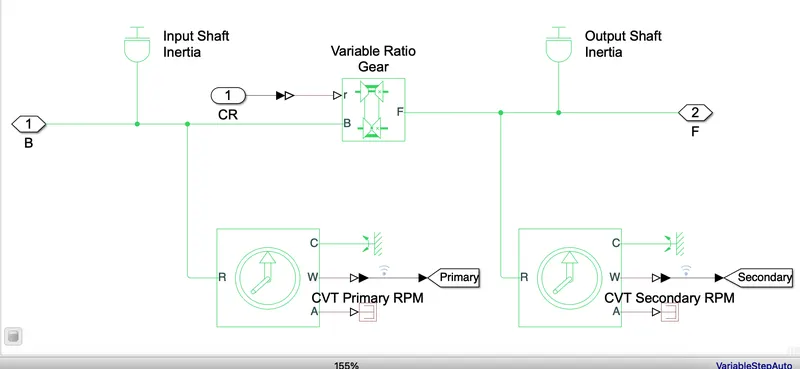
Ports:

• B – Base pulley ore Drive Pulley
• F – Follower Pulley or Driven Pulley
• r – Variable Transmission Ratio (Input).

VEHICLE BODY:

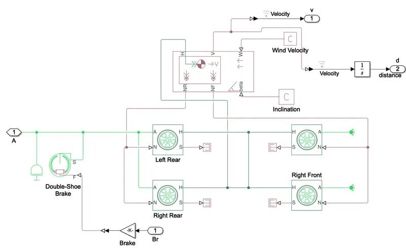
Two – axle vehicle with longitudinal dynamics and motion and adjustable mass, geometry, and drag properties. The vehicle can have the same or a different number of wheels on each axle. For example, two wheels on the front axle and one wheel on the rear axle. The vehicle wheels are assumed identical in size. The vehicle can also have a center of gravity (CG) that is at or below the plane of travel.

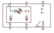
Ports,

• NR – Rear Axle Normal Force (N)
• NF – Front Axle Normal Force (N)
• V – Longitudinal Velocity (m/s)
• W – Head Wind Speed (m/s)
• H – Horizontal Motion
• Beta – Road Incline Angle 9rad)

DOUBLE SHOE BRAKE:

The Double-Shoe Brake block represents a frictional brake with two pivoted rigid shoes that press against a rotating drum to produce a braking action. The rigid shoes sit inside or outside the rotating drum in a diametrically opposed configuration. A positive actuating force causes the rigid shoes to press against the rotating drum. Viscous and contact friction between the drum and the rigid shoe surfaces cause the rotating drum to decelerate.

Ports:

• S – Rotational conserving port associated with the rotating drum shaft
• F – Physical signal input port associated with the applied actuating force.

TIRE:

The vehicle body is connected to 4 tires each per axle to move the vehicle according to the power input to the axle.

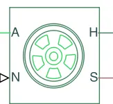
Ports:

• N – Normal Force
• S – Tire Slip
• A – Axle
• H – Mechanical translational port.

BLOCKS USED:

• Signal Builder – To input the Brake, Throttle and CVT Ratio.
• Simulink to PS converter – To convert the Simulink signal to Simscape environment.
• Solver Configuration – To specify the solver parameters before starting the simulation.
• Mechanical Reference – To make sure all the components are clamped to the ground.
• Generic Engine – To run the engine with speed and torque values as input.
• PS to Simulink Converter – To convert Simscape signal to Simulink environment.
• Scope – To view the graph of the parameters for better understanding.
• Display – To view the calculated engine power.
• Inertia – To represent the solid inertia.
• Rotational Motion Sensor – To sense the rotational motion from the engine and give output as RPM.
• Variable Gear Ratio – To vary the speed according to the gear ratios.
• PS Terminator – Terminator for unconnected physical signal outputs.
• Double Shoe Brake – To apply brake to the vehicle when needed.
• PS Constant – Generate constant physical signal.
• Tire – For transportation of the vehicle.
• Rotational Free End – For mechanical component (Tire)
• Vehicle Body – To represent the BAJA ATV model body.
• Custom Measure Gauge – To measure the brake and throttle input.
• Knob – To increase, decrease and vice-versa of throttle and brake inputs.
• Lookup Table – To insert the CVT values from the workspace.
• Simple Gear – To reduce the speed of the engine with pre-defined gear ratio.
• Step – To increase or decrease an input value for a defined time interval.

 SIMULATION PROCESS:

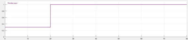
• The throttle signal is generated by signal builder block and inputted to generic engine.
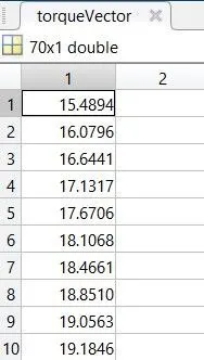
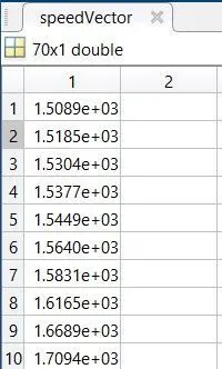
• The torque and speed vector are inputted from the MATLAB workspace.

• The engine will generate the output rpm which can be taken from the crankshaft output. This speed will be given to the Ideal Rotational Motion Sensor to sense the output rpm.
• The same output speed will be given to a simple gear mechanism to reduce the speed where the Gear Ratio is ‘4’.
• Then the output speed from the gear reducer will be given to the Variable Ratio Transmission block (CVT).
• The CVT ratio is provided to the Variable Ratio Transmission (CVT) block through Signal Builder.

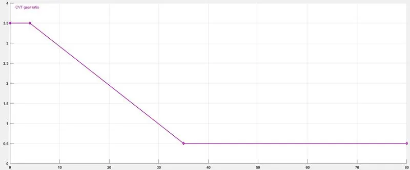
• The speed is controlled by the variable CVT ratios and the controlled output speed is inputted to the vehicle axle.
• The brake signal is generated by the signal builder and inputted to the vehicle body (Double Shoe Brake) for applying the brake to axle.

• The power from the CVT is inputted to the axle and the vehicle accelerates according to the speed.
• Then the Velocity is taken as output from the vehicle body for further analysis.

OUTPUT:

 TORQUE-SPEED PLOT:

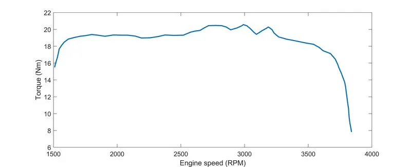
The torque and speed are inputted from the MATLAB workspace window to the generic engine block to generate the output RPM accordingly. This plot is common for all the cases because it’s a default input to the engine.

ENGINE SPEED PLOT:

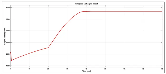
Here we can see the engine rpm generated accordingly w.r.t to the throttle, speed and torque inputs.

ENGINE SPEED vs GEAR REDUCTION SPEED PLOT:

Here we can see that the engine speed is reduced by the Gear Ratio ‘4’. For verification I calculated the maximum RPM.

Maximum RPM (Before Reducing) = 3833 rpm

Gear Ratio = 1:4

We know that,

Driven = 3833/ 4

Driven = 95625RPM

Thus, the reduced maximum rpm is 958.25rpm which can be verified from the plot.

 Driven = Secondary CVT Shaft

 Driver = Primary CVT Shaft

 

 CVT SPEED REDUCTION PLOT:

 

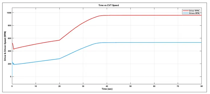
          The engine reduced speed is controlled by various CVT ratios. For verification I had calculated the maximum RPM.

Maximum RPM (Before Reducing) = 958.25rpm

CVT Ratio = 1:1.8

We know that,

Driven = 3833/ 4

Driven = 95625RPM

The reduced maximum rpm is 532.36rpm which can be verified from the plot.

SPEED vs THROTTLE PLOT:

 

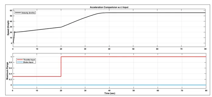
From the graph we can infer that the brake is not applied during the drive cycle and the Throttle is constant (0.3) till 20 sec and being increased from 0.3 to 1 from 20 sec where it remains constant for the rest of the run. With the increase in throttle, the vehicle speed also increases.

ACCELERATION PLOT:

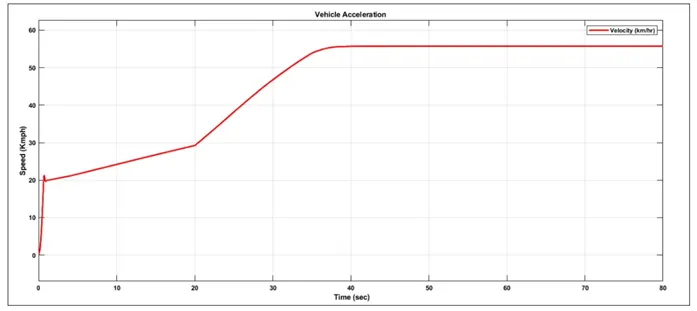
From the above plot, we can infer that the vehicle is accelerated from 0-20kmph and then gradually increases till 30kmph(approx..) and it’s accelerated to 55.74kmph where it remains constant throughout the cycle.

BAJA ATV MODEL WITH DASHBOARD:

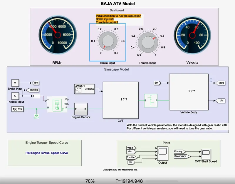
WORKFLOW PROCESS:

The model workflow process is as same as the process of ‘BAJA ATV model without Dashboard’ but the Throttle and Brake inputs are controlled by the user with the Knob. We are also replacing signal builder with two separate constant blocks for Throttle and Brake.

OUTPUT:

 

ENGINE SPEED PLOT:

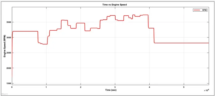
          Here the engine speed is generated according to the inputs like throttle, break, torque and speed vectors. The runtime is not defined so that the Throttle and Break are controlled by the user. The step up is throttle and step down are break inputs.

ENGINE SPEED vs GEAR REDUCTION SPEED PLOT:

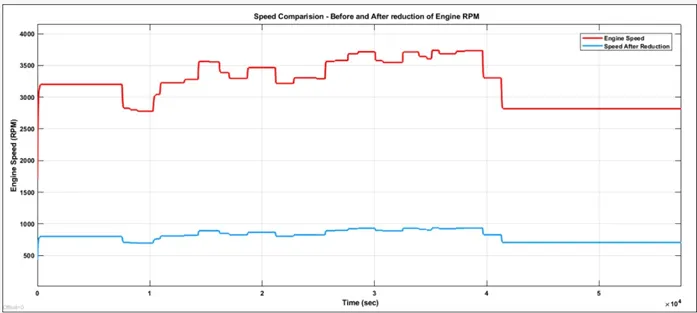
 Here we can see that the engine speed is reduced by the Gear Ratio ‘4’. For verification I calculated the constant RPM (42000 – 50000 sec).

Maximum RPM (Before Reducing) = 2759.3 rpm

Gear Ratio = 1:4

We know that,

Driven = 2759.3/4

Driven = 689.825 RPM

The reduced constant rpm is 689.825 rpm which can be verified from the plot.

CVT SPEED REDUCTION PLOT:

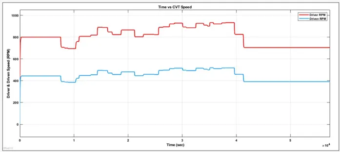
The engine reduced speed is controlled by various CVT Ratios. For verification I had calculated the constant RPM (42000 – 50000 sec)

Maximum RPM (Before Reducing) = 689.825 rpm

CVT Ratio = 1:1.8

We know that,

Driven = 689.825/ 1.8

Driven = 383.23 RPM

The reduced maximum rpm is 383.23 rpm which can be verified from the plot.

SPEED vs THROTTLE PLOT:

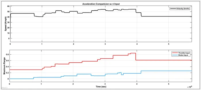
From the graph we can infer that the vehicle is accelerating while throttle is applied (Step Up) and decelerated while break is applied (Step Down).

ACCELERATION PLOT:

 

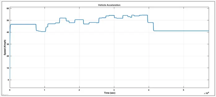
From the graph we can infer that the vehicle is accelerated to 46 kmph initially and then the state changes when the user controls the throttle and brake knobs. The step-up and step-down are acceleration and deceleration respectively. The linear one is the constant speed so no changes in throttle or braking.

SIMULATION OUTPUT:

 

ENGINE SPEED PLOT:

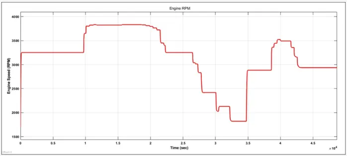
From the graph we can infer that the vehicle was first running at minimum rpm of 3300 rpm and then throttle is applied (step-up) then braking (step-down) then brake is released so that engine rpm is increased then braking is applied. Finally throttle and brake are put to constant of 2900 rpm.

CVT SPEED PLOT:

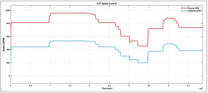
From the above graph we can understand that the throttle is applied (step-up) and then kept constant, then braking is applied (step-down), and finally brake is released so that the engine speed is increased with the increase in throttle input.

INPUT vs VEHICLE SPEED:

 

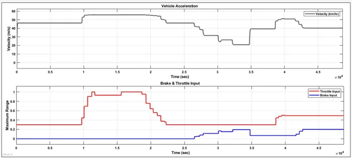
 From the plot we can infer that when throttle is applied the vehicle speed increases and when brake is applied, vehicle speed decreases simultaneously.