Project 1 - Parsing NASA thermodynamic data
File parsing Nasa Thermodynamics
Aim:To write a code in matlab to parsa Nasa thermodynamics data file and then calculate thermodynamic properties of various gas species.
Objectives:
1. To write a function that extracts the 14 co-efficients and calculates the enthalpy, entropy and specific heats for all the species in the data file.The formulae are shown below.
Here R=8.134 is the universal gas constant, T is the temeprature
The FIRST 7 coefficients are HIGH-temperature coefficients and the SECOND 7 coefficients are LOW-temperature coefficients.
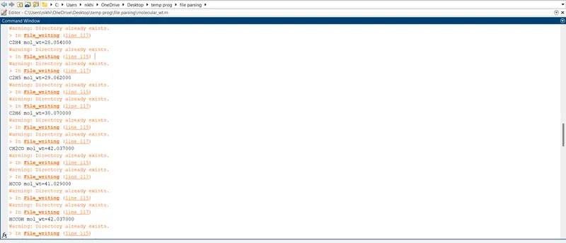
2. To calculate the molecular weight of each species and display it in the command window.
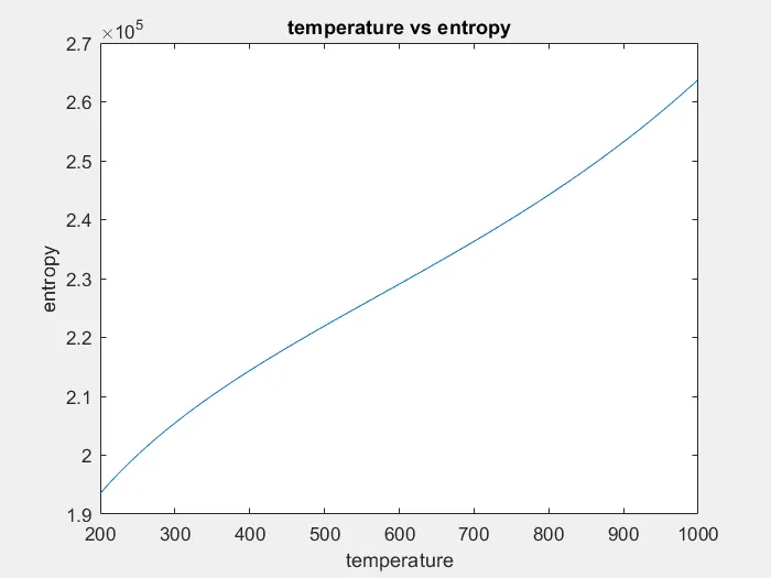
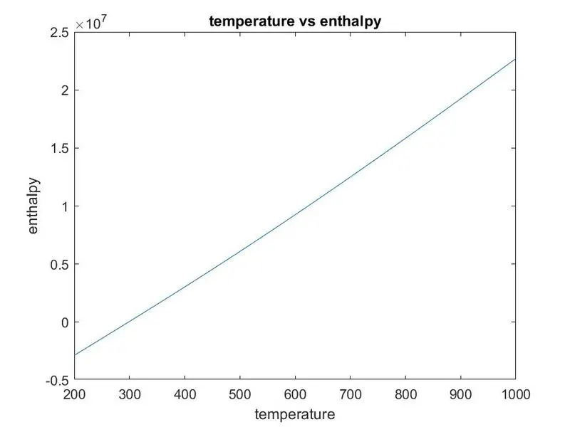
3. To plot the Cp, Enthalpy and Entropy for the local temperature range (low temperature : high temperature) specific for each species.
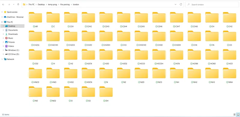
4. To save the plots as images with appropriate names and dump them in separate folders for each species with suitable name. All these should be generated automatically.
5. To write a detailed report to describe your logic.
Theory:
File parsing is a string or symbol either in natural language computer language or data structure conferming to the rules of the former grammer.
Mathematical Equation:
The formulae are shown below.
Here R=8.134 is the universal gas constant, T is the temeprature
The FIRST 7 coefficients are HIGH-temperature coefficients and the SECOND 7 coefficients are LOW-temperature coefficients.
Program for file parsing:
File parsing function:
clc
close all
%clear all
f1=fopen('thermo.dat','r');
%reading header information
fgetl(f1);
%global temperature
tline=fgetl(f1);
a=strsplit(tline,' ');
global_low_temp=str2double(a{2});
global_mid_temp=str2double(a{3});
global_high_temp=str2double(a{4});
%neglecting the next 3 lines
fgetl(f1);
fgetl(f1);
fgetl(f1);
%reading species block
%line1
for i=1:53
t_line2=fgetl(f1);
s=strsplit(t_line2,' ');
species_name=s{1};
A=strfind(t_line2,'G');
temp_values=t_line2(A+4:length(t_line2));
B=strsplit(temp_values,' ');
local_low_temp=str2double(B{1});
local_med_temp=str2double(B{2});
local_high_temp=str2double(B{3});
t_line=fgetl(f1);
b=strfind(t_line,'E');
%1st coeff
b1=t_line(1:b(1)+3);
b1=str2double(b1);
%2nd coeff
b2=t_line(b(1)+4:b(2)+3);
b2=str2double(b2);
%3rd cooeff
b3=t_line(b(2)+4:b(3)+3);
b3=str2double(b3);
% 4th coeff
b4=t_line(b(3)+4:b(4)+3);
b4=str2double(b4);
%5th coeff
b5=t_line(b(4)+4:b(5)+3);
b5=str2double(b5);
%line2
line2=fgetl(f1);
%6thcoeff
b6=line2(1:b(1)+3);
b6=str2double(b6);
%7th coeff
b7=line2(b(1)+4:b(2)+3);
b7=str2double(b7);
%8th coeff
b8=line2(b(2)+4:b(3)+3);
b8=str2double(b8);
%9th coeff
b9=line2(b(3)+4:b(4)+3);
b9=str2double(b9);
%10th coeff
b10=line2(b(4)+4:b(5)+3);
b10=str2double(b10);
%line3
line3=fgetl(f1);
%11th coeff
b11=line3(1:b(1)+3);
b11=str2double(b11);
%12th coeff
b12=line3(b(1)+4:b(2)+3);
b12=str2double(b12);
%13th coeff
b13=line3(b(2)+4:b(3)+3);
b13=str2double(b13);
%14th coeff
b14=line3(b(3)+4:b(4)+3);
b14=str2double(b14);
%universal gas constant
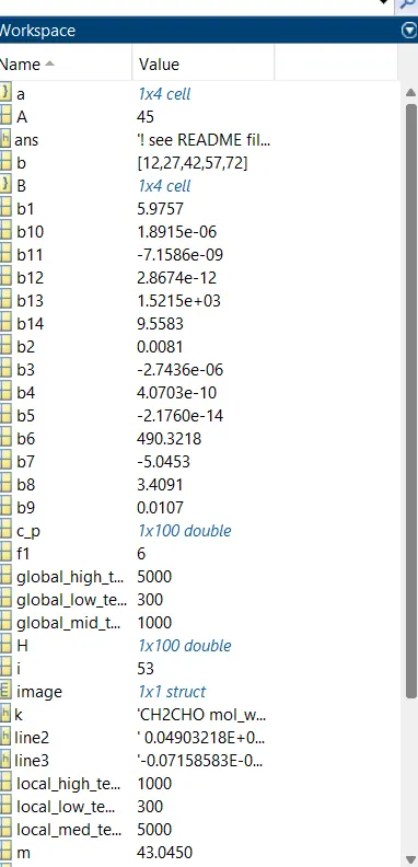
R=8314;
t=linspace(local_low_temp,local_high_temp,100);
%calculate
% specific heat by creating function
c_p=specific_heat(b1,b,b3,b4,b5,b6,b7,b8,b9,b10,b11,b12,b13,b14,local_low_temp,local_med_temp,local_high_temp,t,R);
%enthalpy by creating function
H=enthalpy(b1,b2,b3,b4,b5,b6,b7,b8,b9,b10,b11,b12,b13,b14,local_low_temp,local_med_temp,local_high_temp,t,R);
%entrophy by creating function
S=Entrophy(b1,b2,b3,b4,b5,b6,b7,b8,b9,b10,b11,b12,b13,b14,local_low_temp,local_med_temp,local_high_temp,t,R);
%creating a folder
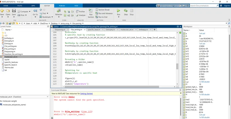
mkdir('london')
cd('london')
mkdir(species_name)
cd(species_name)
%plotting for
%temperature vs specific heat
figure(1)
plot(t,c_p)
xlabel('temperature')
ylabel('specific heat')
title('temperature vs specific heat')
image=getframe(gcf);
imwrite(image.cdata,'t vs cp.png')
saveas(1,'specific heat','jpg')
%temperature vs enthalpy
figure(2)
plot(t,H)
xlabel('temperature')
ylabel('enthalpy')
title('temperature vs enthalpy')
image=getframe(gcf);
imwrite(image.cdata,'t vs H.png')
saveas(2,'enthalpy','jpg')
%temperature vs entropy
figure(3)
plot(t,S)
xlabel('temperature')
ylabel('entropy')
title('temperature vs entropy')
image=getframe(gcf);
imwrite(image.cdata,'t vs S.png')
saveas(3,'entropy','jpg')
cd ..
cd ..
%calculating molecular mass
[m]=molecular_wt(species_name);
k=sprintf('%s mol_wt=%f',species_name,m);
disp(k)
end
Fuction for Enthalpy:
%for enthalpy
function [H]=enthalpy(b1,b2,b3,b4,b5,b6,~,b8,b9,b10,b11,b12,b13,~,~,local_mid_temp,~,t,R)
if (t>local_mid_temp)
H=(b1+((b2.*t)/2)+((b3.*(t.^2))/3)+((b4.*(t.^3))/4)+((b5.*(t.^4))/5)+(b6./t)).*t*R;
else
H=(b8+((b9.*t)/2)+((b10.*(t.^2))/3)+((b11.*(t.^3))/4)+((b12.*(t.^4))/5)+(b13./t)).*t*R;
end
Function for Entrophy:
% clc
% close all
% clear all
%Function for file_writing
%for Entropy
function [S]=Entrophy(b1,b2,b3,b4,b5,~,b7,b8,b9,b10,b11,b12,~,b14,~,local_mid_temp,~,t,R)
if (t>local_mid_temp)
S=((b1.*logt)+(b2.*t)+((b3.*(t.^2))/2)+((b4.*(t.^3))/3)+(b5.*(t.^4))+b7);
else
S=((b8.*log(t))+(b9.*t)+((b10.*(t.^2))/2)+((b11.*(t.^3))/3)+(b12.*(t.^4))+b14)*R;
end
end
Function for Specific heat:
% clc
% close all
% clear all
%Function for file_writing
%for specific heat
function [c_p]=specific_heat(b1,b2,b3,b4,b5,~,~,b8,b9,b10,b11,b12,~,~,~,local_mid_temp,~,t,R)
if (t>local_mid_temp)
c_p=R*(b1+(b2.t)+(b3.*(t.^2))+(b4.*(t.*3))+(b5.*(t.^4)));
else
c_p=R*(b8+(b9.*t)+(b10.*(t.^2))+(b11.*(t.^3))+(b12.*(t.^4)));
end
Function for Molecular weight:
%for molecular weight
function [m]=molecular_wt(species_name)
atomic_mass=[15.999,1.008,12.011,14.007,39.948];
elements=['O','H','C','N','A'];
mol_wt=0;
for i=1:length(species_name)
for j=1:length(elements)
if strcmpi(species_name(i),elements(j))
mol_wt=mol_wt+atomic_mass(j);
z=j;
end
end
t=str2double(species_name(i));
if(t>1)
mol_wt=mol_wt+(atomic_mass(z)*(t-1));
end
end
m=mol_wt;
end
Outputs:
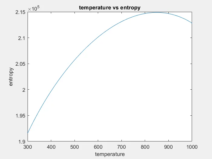
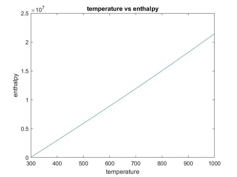
N2
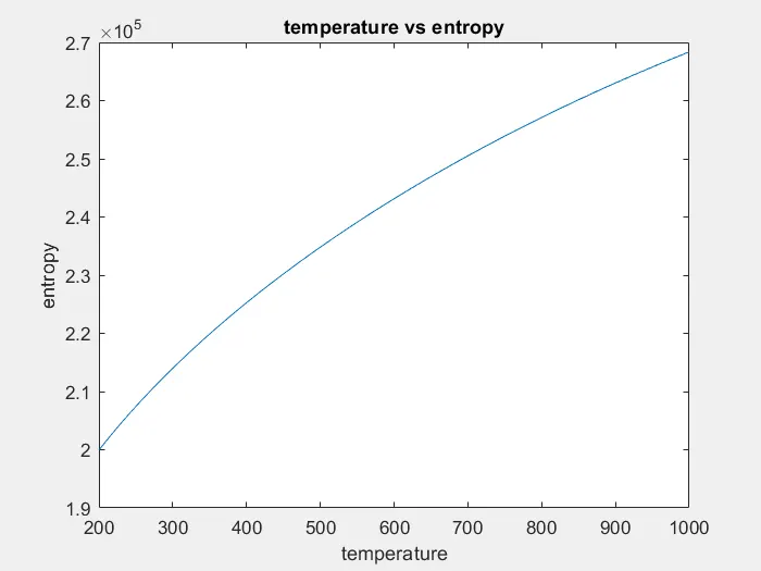
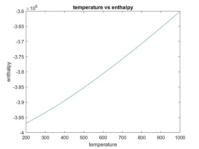
CO2:
O2:
Error faced:
Location of the files saved:
Molecular Weight for each elements are shown in command window:
Results:
- The program and code for file parsing is written and executed.
- The graph for N2,CO2,O2 is plotted
- Molecular weights for every element is genrated and found
- Files are created in a folder.