Project 1 - Parsing NASA thermodynamic data

1. File Pursing coding

clear all
close all
clc

% Here R is the universal gas constant,
f1=fopen('THERMO.dat','r');

% header extract the value of global temperature
t_1 = fgetl(f1);
t_2 = fgetl(f1);

globel_temp = strsplit(t_2,' ');
globel_temp_low = str2double (globel_temp{2});
globel_temp_medium = str2double (globel_temp{3});
globel_temp_high = str2double (globel_temp{4});

% leaving ext three lines as they are part of header
fgetl(f1)
fgetl(f1)
fgetl(f1)

% Before start we create a folder at desired location



% Now we can access data to be operated
for i=1:53


 
    tline_1str= fgetl(f1);
    tline_1= strsplit(tline_1str);
    component= tline_1{1};
   
    low_temp = str2double(tline_1{end-3});
    medium_temp = str2double(tline_1{end-1});
    high_temp = str2double(tline_1{end-2});

    % Extracting Coefficients
    tline_2str = fgetl(f1);
    a= strfind(tline_2str,'E');
    a1_str = tline_2str(1:a(1)+3);   % coefficient is extracted as string
    a2_str= tline_2str(a(1)+4:a(2)+3); 
    a3_str = tline_2str(a(2)+4:a(3)+3);
    a4_str = tline_2str(a(3)+4:a(4)+3);
    a5_str = tline_2str(a(4)+4:a(5)+3);

    a1 = str2double(a1_str);
    a2 = str2double(a2_str);
    a3 = str2double(a3_str);
    a4 = str2double(a4_str);
    a5 = str2double(a5_str);

    % same procedure for next line
    tline_3str=fgetl(f1);
    b=strfind(tline_3str,'E');

    a6_str = tline_3str(1:b(1)+3);
    a7_str = tline_3str(b(1)+4:b(2)+3);
    a8_str = tline_3str(b(2)+4:b(3)+3);
    a9_str = tline_3str(b(3)+4:b(4)+3);
    a10_str = tline_3str(b(4)+4:b(5)+3);

    a6 = str2double(a6_str); % saving co-efficient as number
    a7 = str2double(a7_str);
    a8 = str2double(a8_str);
    a9 = str2double(a9_str);
    a10 = str2double(a10_str);

    % For next line we have only four co-efficients
    tline_4str=fgetl(f1);
    c=strfind(tline_4str,'E');

    a11_str = tline_4str(1:c(1)+3);
    a12_str = tline_4str(c(1)+4:c(2)+3);  % co-efficient is extracted as string
    a13_str = tline_4str(c(2)+4:c(3)+3);
    a14_str = tline_4str(c(3)+4:c(4)+3);

    a11 = str2double(a11_str); % saving co-efficient as number
    a12 = str2double(a12_str);
    a13 = str2double(a13_str);
    a14 = str2double(a14_str);

    % calculating CP, H and S.
    local_temp_range = linspace(low_temp,high_temp,50);

R=8.314;
  for i = 1:length(local_temp_range)

        T = local_temp_range(i);
        if T> medium_temp 
     
    CP(i)= R*(a1+a2*T+a3*(T^2)+a4*(T^3)+a5*(T^4));
   H(i) = (R*T)*(a1+(a2*T)/2+(a3*T^2)/3+(a4*T^3)/4+(a5*T^4)/5+a6/T);
    S(i) = R*(a1*log(T)+a2*T+(a3*T^2)/2+(a4*T^3)/3+(a5*T^4)/4+a7);
        else 

    CP(i) = R*(a8+a9*T+a10*(T^2)+a11*(T^3)+a12*(T^4));
    H(i)  = (R*T)*(a8+(a9*T)/2+(a10*T^2)/3+(a11*T^3)/4+(a12*T^4)/5+a13/T);
    S(i)  = R*(a8*log(T)+a9*T+(a10*T^2)/2+(a11*T^3)/3+(a12*T^4)/4+a14);

    end
        end


   % plot for CP,H,S
   figure(1)
   plot(local_temp_range,CP);
   xlabel('Temperature');
   ylabel('specific heat')
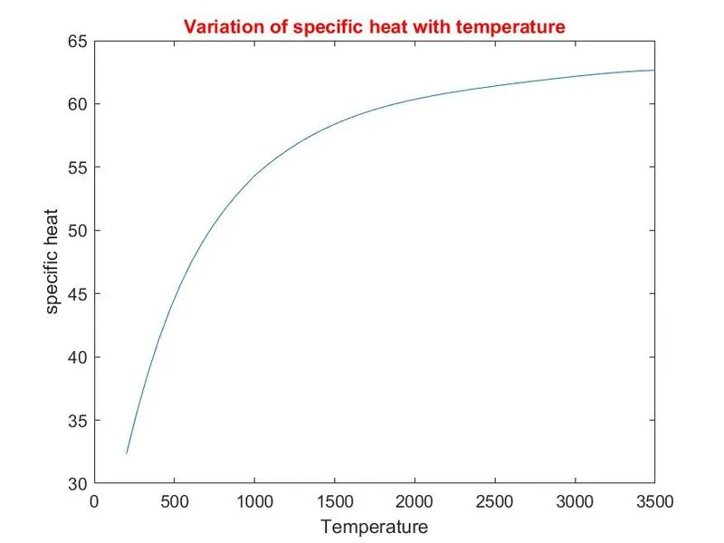
   title('Variation of specific heat with temperature','color','r');

   figure(2)
   plot(local_temp_range,H);
   xlabel('Temperature');
   ylabel('Entholpy');
   title('Variation of enthalpy with temperature','color','R')

   figure(3)
   plot(local_temp_range,S);
   xlabel('Temperature')
   ylabel('Entropy');
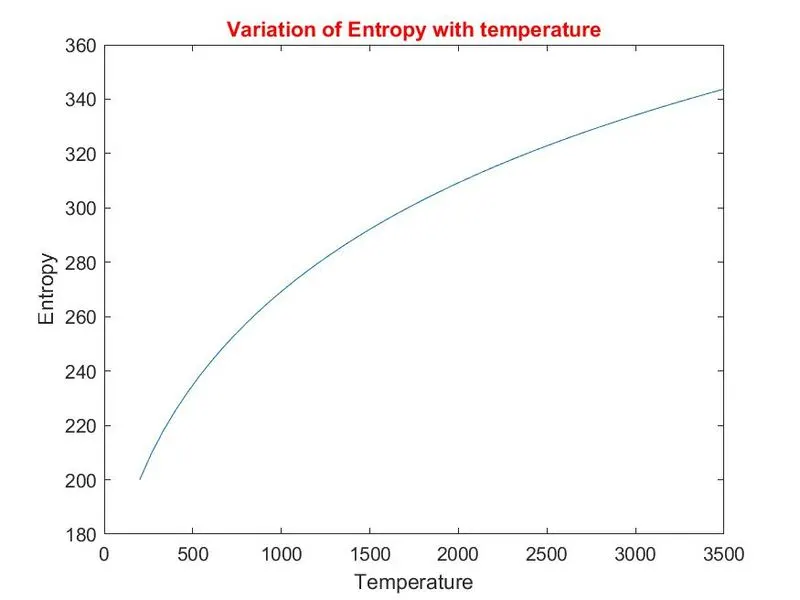
   title('Variation of Entropy with temperature','color','r');

   mkdir(component)
   cd(component)
   saveas(1,'Sp_Heat.jpg')
      saveas(2,'Enthalpy.jpg')
      saveas(3,'Entropy.jpg')
      
    cd ..
   % calculating molecular weight

   mole_weight = molecular_weight(component);
   fprintf('molecular_weight of %S is %d, \n',component,mole_weight)

end

2. Molecular weight function

  function mole_weight = molecular_weight(component)


 %[O,H,C,S,N,AR]=deal(16,1,12,32,14,39.948);
Elements=['O','H','C','N','A'];
Atomic_weight=[16,1,12,14,40];
% weight=[O H C S N AR]

mole_weight=0;
for i = 1:length(component)
    for j = 1:length(Elements)
        if strcmp(component(i),Elements(j))
        mole_weight=mole_weight+Atomic_weight(j);
        position=j;
        end
    end


m=str2num(component(i));
if m>1;
mole_weight=mole_weight+Atomic_weight(position)*(m-1)
end
end 

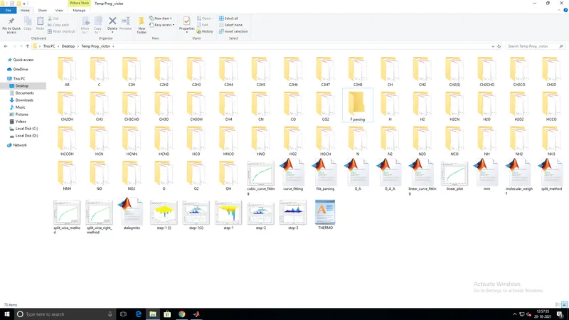
3. species folder images

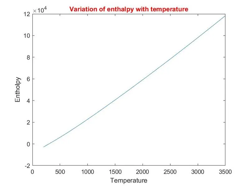
4. O2 - plots

i, Enthalpy

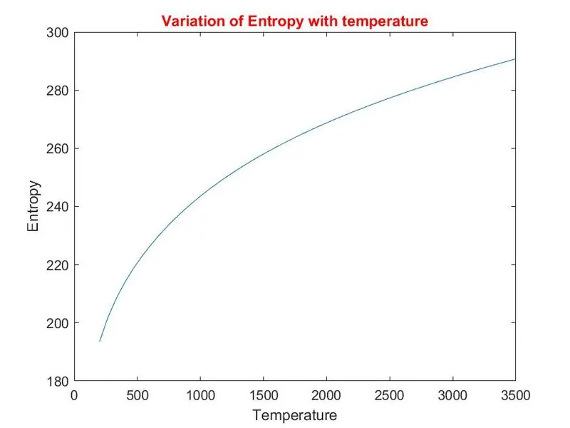
ii,. entropy

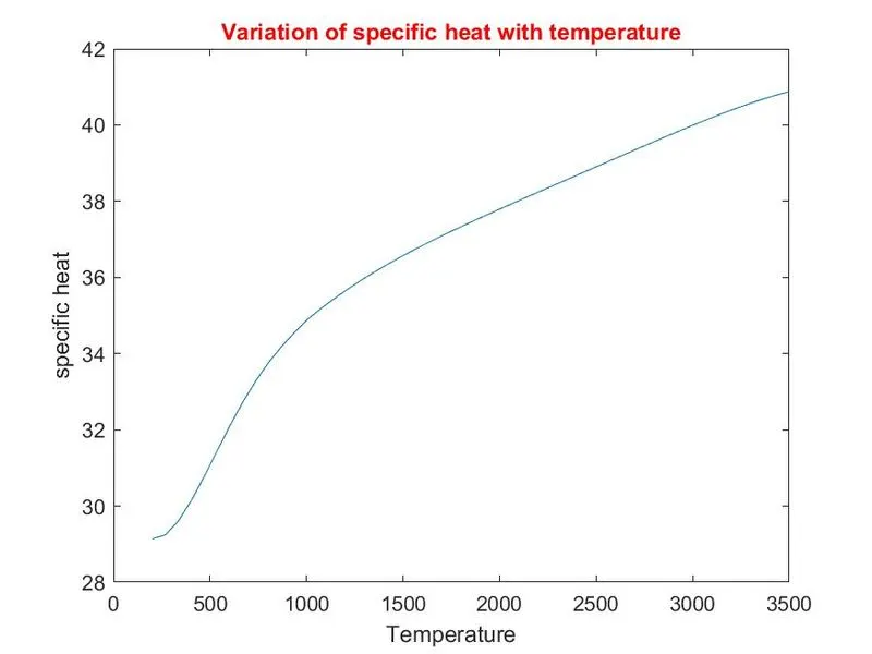
iii, specfic heat

2. N2 - plots

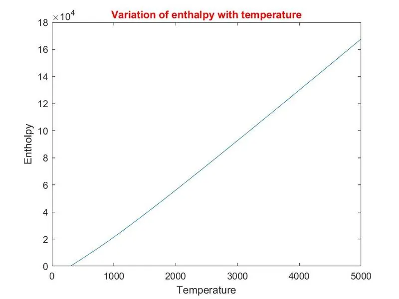
i, Enthalpy

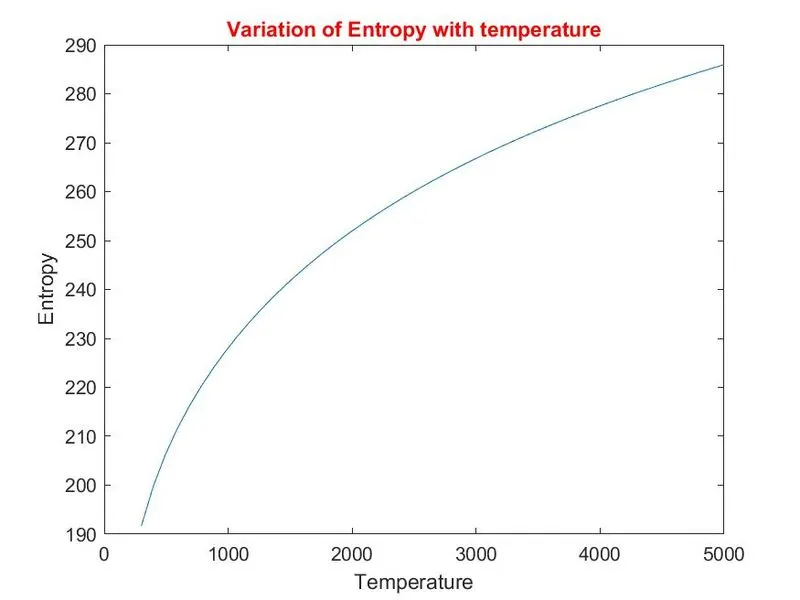
ii, Entropy

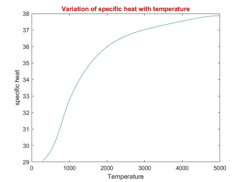
iii, Specfic heat

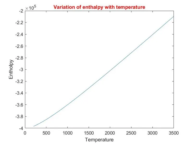
3. Co2 - plots

i, Enthalpy

ii, Entropy

iii, Specific heat

Explanation:

1. First the Thermo.data file is opened to read using fopen command and is saved in a specfic file identifier.

2. Line.no. 5 & 6 - (R - universal constant) & put the name of f1.

3.Line.no. 8-15 - header extract the value of global temperature (low, medium & high)

4.Line.no.17 -20 - next three lines are skipped, as they are only part of header, using (fgetl).

5.Line. no. 27 -137 - we can access data to be operated function.

6. The function details are given below,

The total species are 53, so we using the function of (i=1:53)

7. Line.no. 31-37 - To extract the temperature value as the same of thermodata reference. so using strsplit command and segregate the value. (low, medium, high) temperature for first species.

8. Line.no.39-52 - Extracting co-efficient of first species, using strfind to identify the position of 'E'. and extract the value's as the same given inputs.

9. Line.no.54-82 - The remaining species as follow by the same procedure as mention in above.

10. Line.no.84-103 - calculating CP,H & S. Followed by the formula's as given in question.

11. Line.no.106-123 - Plot for (enthalpy, entropy and specfic heat) in this order in all species.

12. Line.no.125-131 - To create a folder in added the plot for individual species upto 53.

13. Line.no.132-137 + molecular weight function - to find a molecular weight using new function and derive the molecules weight for using comparsion commands for strcmp (components and elements).

conclusion:

Using matlab code, the necessary coefficients required to evaluate various thermodynamic parameters for different species are extracted from NASA thermodynamic data file. The specific heat, enthalpy and entropy for all the species are calculated and plotted against local temperature range. The molecular weight is calculated for all the species.