Project 1 - Parsing NASA thermodynamic data
AIM: To optimise the stalagmite function and find the global maxima of the function.
OBJECTIVES OF THE PROJECT: Explaining the concept of genetic algorithm and also explain the syntax for ga in MATLAB. Plot graphs for all 3 studies and for F maximum vs no. of iterations.
INTRODUCTION: A Genetic Algorithm is a search experiential that is stimulated by Charles Darwin’s theory of natural evolution. This algorithm reproduces the process of natural selection where the appropriate individuals are selected for reproduction in order to produce offspring of the next generation. The genetic algorithm is a technique for solving both constrained and unconstrained optimization problems that are based on natural selection, the process that drives biological evolution. The genetic algorithm constantly modifies the population size of individual solutions.
Phases in Genetic Algorithm
- Initialization of Population (Coding) The code generates its random population of defined size and from that population the code evaluates the fitness of the members of the population according to which it forms new population based on no. of iterations performed.
- Fitness Function It is that function which we have to optimize and its optimization is done with the help of number of generations which have been formed by the code accordance with the fitness value of each member generated, these fitness values are used for the reproduction of the children.
1.Selection The idea of the selection phase is to select the fittest individuals and let them pass their genes to the next generation. The main goal of this phase is to find the region where the chances of getting the best solution are more. Inspiration for this is from the survival of the fittest. It should be a balance between exploration and exploitation of search space. GA tries to move the genotype to higher fitness in the search space. Too strong fitness selection bias can lead to sub-optimal solutions. Too little fitness bias selection results in unfocused search.
- Reproduction Generation of offspring happen in 2 ways: Crossover Mutation 1.
- a) Crossover
Crossover is the most significant stage in the genetic algorithm. During crossover, a random point is selected while mating a pair of parents to generate offspring. There are 3 major types of crossover. Single Point Crossover: A point on both parents’ chromosomes is picked randomly, and designated a ‘crossover point’.
Two-Point Crossover: Two crossover points are picked randomly from the parent chromosomes. Uniform Crossover:
In a uniform crossover, typically, each bit is chosen from either parent with equal probability. The new offspring are added to the population.
- b) Mutation
In a few new offspring formed, some of their genes can be subjected to a mutation with a low random probability. This indicates that some of the bits in the bit chromosome can be flipped. Mutation happens to take care of diversity among the population and stop premature convergence.
Syntax for GA:
[x,fval ,exitflag ,output ,population ,scores]= ga(func,nvars,A,b,Aeq,Beq,lb,ub,nonlcon,Intcon,options)
x = optimum solution exitflag = reason ga stopped output= information about optimization process population=final population scores= final scores f=ga(fun,nvars,A,b,[],[],lb,ub,nonlcon,IntCon,options)
fun - fitness function.
nvars- number of variables,
A,b= Linear inequality constraints
Aeq,beq=Linear equality constraints lb- Lower bound(limit),
ub- Upper bound(limit),
nonlcon : Use for nonlinear constraints
IntCon : to get solution in integer. options- To set population size minimize with non-default options
clear all
close all
clc
%getting the data file
f1=fopen('THERMO.dat','r');
fgetl(f1)
%reading the header information
A=fgetl(f1);
A=strsplit(A,' ');
global_low_temp=str2num(A{2});
global_mid_temp=str2num(A{3});
global_high_temp=str2num(A{4});
%skipping next three lines
for i=1:3
fgetl(f1);
end
%reading the species
for i=1:53
header=fgetl(f1);
x=strsplit(header,' ');
species_name=(x{1});
z=length(x);
local_low_temp=str2double(x{z-3});
local_high_temp=str2double(x{z-2});
local_mid_temp=str2double(x{z-1});
t1=local_low_temp;
t2=local_mid_temp;
t3=local_high_temp;
%getting first line coeffecients (a1-a5)
line_1=fgetl(f1);
a=strfind(line_1,'E');
a1=str2double(line_1(1:a(1)+3));
a2=str2double(line_1(a(1)+4:a(2)+3));
a3=str2double(line_1(a(2)+4:a(3)+3));
a4=str2double(line_1(a(3)+4:a(4)+3));
a5=str2double(line_1(a(4)+4:a(5)+3));
%getting second line coeffeceints (a6-a10)
line_2=fgetl(f1);
a_1=strfind(line_2,'E');
a6=str2num(line_2(1:a_1(1)+3));
a7=str2double(line_2(a_1(1)+4:a_1(2)+3));
a8=str2double(line_2(a_1(2)+4:a_1(3)+3));
a9=str2double(line_2(a_1(3)+4:a_1(4)+3));
a10=str2double(line_2(a_1(4)+4:a_1(5)+3));
%getting third line coeffeceints (a10-a14)
line_3=fgetl(f1);
a_2=strfind(line_1,'E');
a11=str2double(line_3(1:a_2(1)+3));
a12=str2double(line_3(a_2(1)+4:a_1(2)+3));
a13=str2double(line_3(a_2(2)+4:a_1(3)+3));
a14=str2double(line_3(a_2(3)+4:a_1(4)+3));
%creating folder
mkdir(['C:\Users\Student\Desktop\RAJKUMAR\MATLAB\file parsing\images\',species_name]);
T=linspace(t1,t3,1000);
R=8.314;
% to get array of specific heat, enthalpy and entropy
for k=1:length(T)
% to compare the species temperature to assign the coeffeceints
%a1-a7 (high temperature coeffeceints), a8-a14(low temperature coeffecients)
if T(k)>t2
%high temperature coeffeceints.
cp=(a1+a2.*T+a3.*T.^2+a4.*T.^3+a5.*T.^4)*R;
H=(a1+(a2.*T)/2+(a3.*T.^2)/3+(a4.*T.^3)/4+(a5.*T.^4)/5+(a6./T))*R.*T;
S=a1.*log(T)+a2.*T+(a3.*T.^2)/2+(a4.*T.^3)/3+(a5.*T.^4)/4+a7;
else
%low temperature coeffecients
cp=(a8+a9.*T+a10.*T.^2+a11.*T.^3+a12.*T.^4)*R;
H=(a8+(a9.*T)/2+(a10.*T.^2)/3+(a11.*T.^3)/4+(a12.*T.^4)/5+(a13./T))*R.*T;
S=a8.*log(T)+a9.*T+(a10.*T.^2)/2+(a11.*T.^3)/3+(a12.*T.^4)/4+a14;
end
end
%plotting the graphs
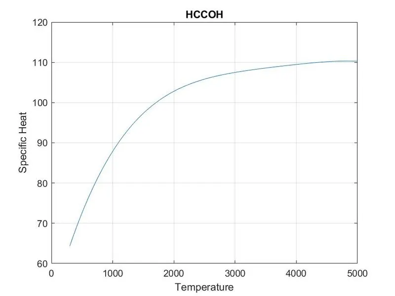
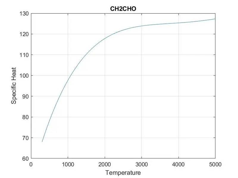
figure(1);
plot(T,cp);
grid on ;
title(species_name);
xlabel('Temperature');
ylabel('Specific Heat');
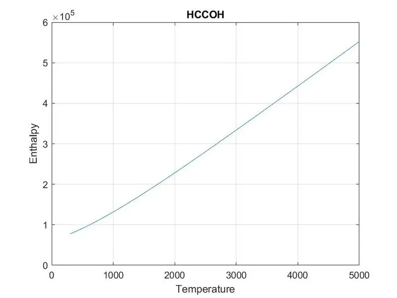
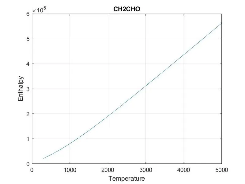
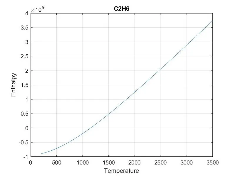
figure(2);
plot(T,H);
grid on ;
title(species_name);
xlabel('Temperature');
ylabel('Enthalpy');
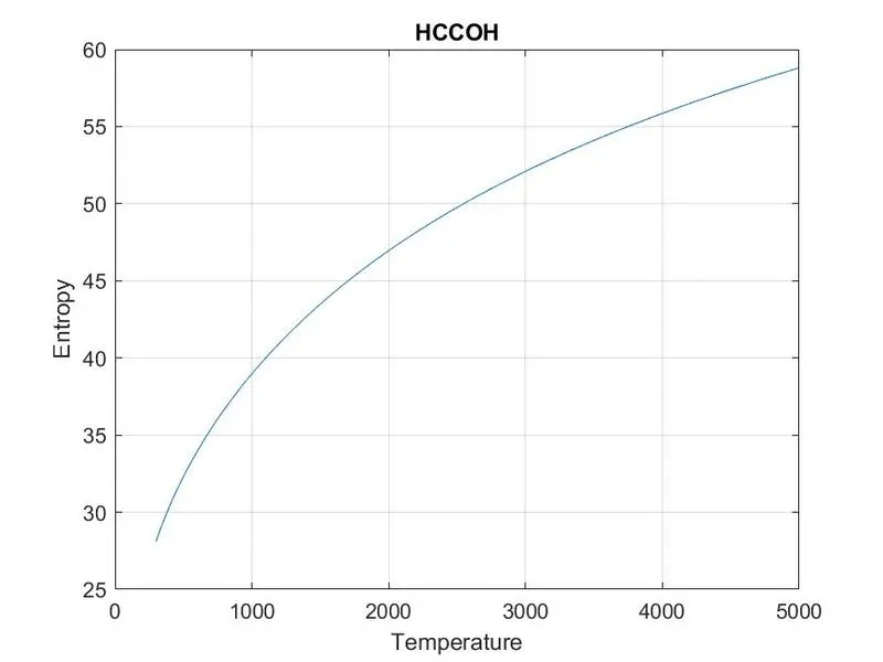
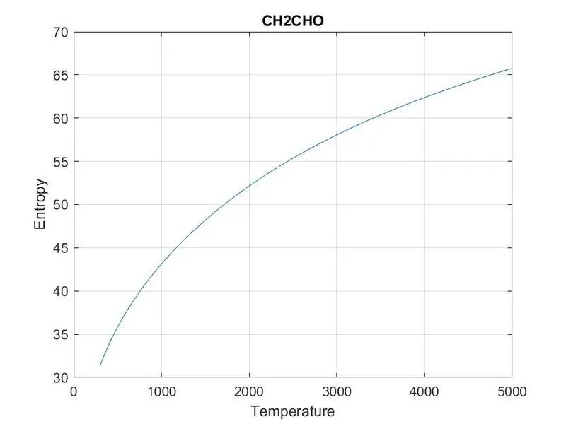
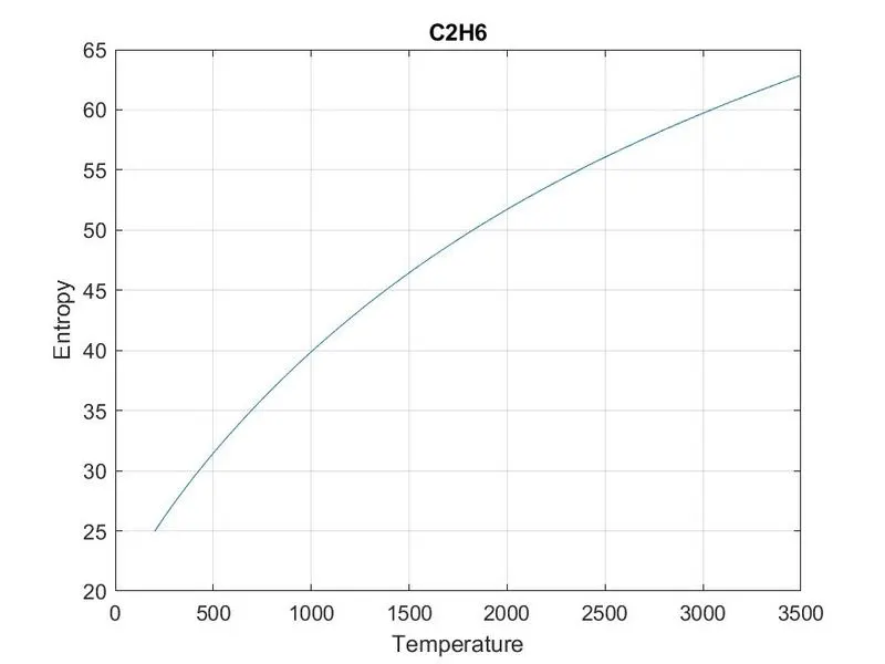
figure(3);
plot(T,S);
grid on ;
title(species_name);
xlabel('Temperature');
ylabel('Entropy');
%changing the directory and saving the file
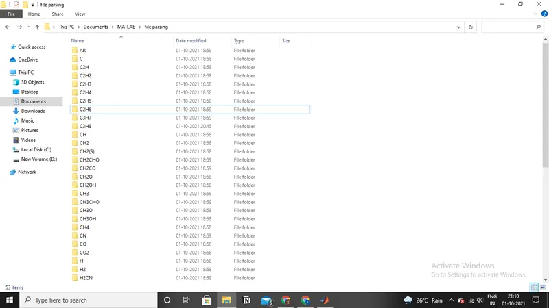
cd=(['C:\Users\Student\Desktop\RAJKUMAR\MATLAB\file parsing\images\',species_name]);
saveas(1,'specific heat','jpg');
saveas(2,'enthalpy','jpg');
saveas(3,'entropy','jpg');
%molecular_masscalculation
elements=['H','C','O','N','A'];
atomic_weight=[1.0079 12.0107 15.999 14.0067 39.948];
mol_mass=0;
for l=1:length(species_name)
for m=1:length(atomic_weight)
if strcmp(species_name(l),elements(m))
mol_mass=mol_mass+atomic_weight(m);
position=m;
end
end
n=str2double(species_name(l));
if n>1
mol_mass=mol_mass+atomic_weight(position)*(n-1);
end
end
sprintf('Molecular Weight of %s:%f u',species_name,mol_mass)
end
fclose(f1)
Code explanation
clear all
close all
clc
%getting the data file
f1=fopen('THERMO.dat','r');
fgetl(f1)
%reading the header information
A=fgetl(f1);
A=strsplit(A,' ');
global_low_temp=str2num(A{2});
global_mid_temp=str2num(A{3});
global_high_temp=str2num(A{4});
%skipping next three lines
for i=1:3
fgetl(f1);
end
%reading the species
for i=1:53
header=fgetl(f1);
x=strsplit(header,' ');
species_name=(x{1});
z=length(x);
local_low_temp=str2double(x{z-3});
local_high_temp=str2double(x{z-2});
local_mid_temp=str2double(x{z-1});
t1=local_low_temp;
t2=local_mid_temp;
t3=local_high_temp;
%getting first line coeffecients (a1-a5)
line_1=fgetl(f1);
a=strfind(line_1,'E');
a1=str2double(line_1(1:a(1)+3));
a2=str2double(line_1(a(1)+4:a(2)+3));
a3=str2double(line_1(a(2)+4:a(3)+3));
a4=str2double(line_1(a(3)+4:a(4)+3));
a5=str2double(line_1(a(4)+4:a(5)+3));
%getting second line coeffeceints (a6-a10)
line_2=fgetl(f1);
a_1=strfind(line_2,'E');
a6=str2num(line_2(1:a_1(1)+3));
a7=str2double(line_2(a_1(1)+4:a_1(2)+3));
a8=str2double(line_2(a_1(2)+4:a_1(3)+3));
a9=str2double(line_2(a_1(3)+4:a_1(4)+3));
a10=str2double(line_2(a_1(4)+4:a_1(5)+3));
%getting third line coeffeceints (a10-a14)
line_3=fgetl(f1);
a_2=strfind(line_1,'E');
a11=str2double(line_3(1:a_2(1)+3));
a12=str2double(line_3(a_2(1)+4:a_1(2)+3));
a13=str2double(line_3(a_2(2)+4:a_1(3)+3));
a14=str2double(line_3(a_2(3)+4:a_1(4)+3));
%creating folder
mkdir(['C:\Users\Student\Desktop\RAJKUMAR\MATLAB\file parsing\images\',species_name]);
T=linspace(t1,t3,1000);
R=8.314;
% to get array of specific heat, enthalpy and entropy
for k=1:length(T)
% to compare the species temperature to assign the coeffeceints
%a1-a7 (high temperature coeffeceints), a8-a14(low temperature coeffecients)
if T(k)>t2
%high temperature coeffeceints.
cp=(a1+a2.*T+a3.*T.^2+a4.*T.^3+a5.*T.^4)*R;
H=(a1+(a2.*T)/2+(a3.*T.^2)/3+(a4.*T.^3)/4+(a5.*T.^4)/5+(a6./T))*R.*T;
S=a1.*log(T)+a2.*T+(a3.*T.^2)/2+(a4.*T.^3)/3+(a5.*T.^4)/4+a7;
else
%low temperature coeffecients
cp=(a8+a9.*T+a10.*T.^2+a11.*T.^3+a12.*T.^4)*R;
H=(a8+(a9.*T)/2+(a10.*T.^2)/3+(a11.*T.^3)/4+(a12.*T.^4)/5+(a13./T))*R.*T;
S=a8.*log(T)+a9.*T+(a10.*T.^2)/2+(a11.*T.^3)/3+(a12.*T.^4)/4+a14;
end
end
%plotting the graphs
figure(1);
plot(T,cp);
grid on ;
title(species_name);
xlabel('Temperature');
ylabel('Specific Heat');
figure(2);
plot(T,H);
grid on ;
title(species_name);
xlabel('Temperature');
ylabel('Enthalpy');
figure(3);
plot(T,S);
grid on ;
title(species_name);
xlabel('Temperature');
ylabel('Entropy');
%changing the directory and saving the file
cd=(['C:\Users\Student\Desktop\RAJKUMAR\MATLAB\file parsing\images\',species_name]);
saveas(1,'specific heat','jpg');
saveas(2,'enthalpy','jpg');
saveas(3,'entropy','jpg');
%molecular_masscalculation
elements=['H','C','O','N','A'];
atomic_weight=[1.0079 12.0107 15.999 14.0067 39.948];
mol_mass=0;
for l=1:length(species_name)
for m=1:length(atomic_weight)
if strcmp(species_name(l),elements(m))
mol_mass=mol_mass+atomic_weight(m);
position=m;
end
end
n=str2double(species_name(l));
if n>1
mol_mass=mol_mass+atomic_weight(position)*(n-1);
end
end
sprintf('Molecular Weight of %s:%f u',species_name,mol_mass)
end
fclose(f1)
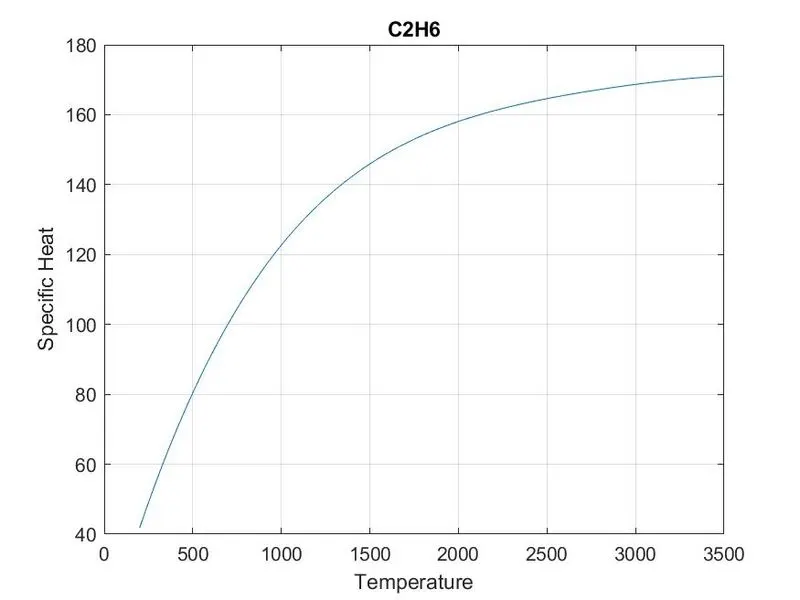
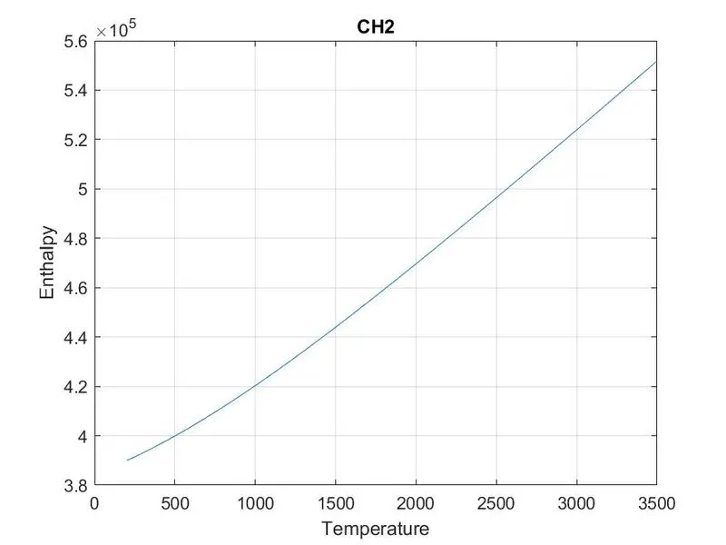
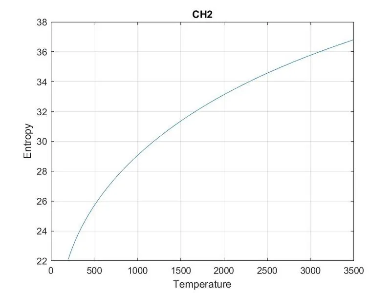
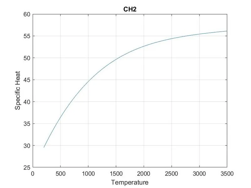
outputs