Parsing NASA thermodynamic data

Parsing Nasa Thermodynamic data.

Aim: The Aim of this project is to extract Temperature and coefficient data from each element and find their Specific heat, Enthalpy, Entropy, and Molecular mass.

Objective:

• Separate and capture the Low-temperature coefficients and high temperature for each of the Elements.
• Separate the Local low temperature and local high temperature for each of the elements.
• Calculate the Enthalpy, Entropy, and Specific heat using the given formula.
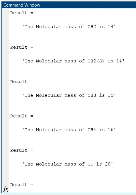
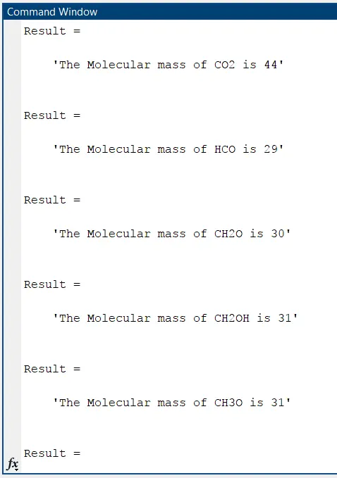
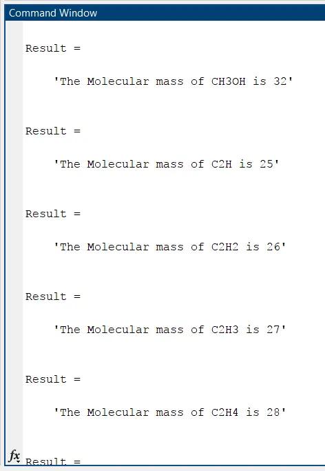
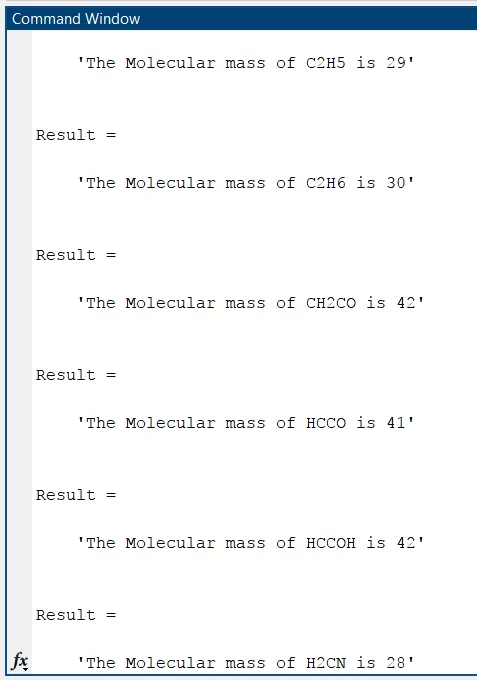
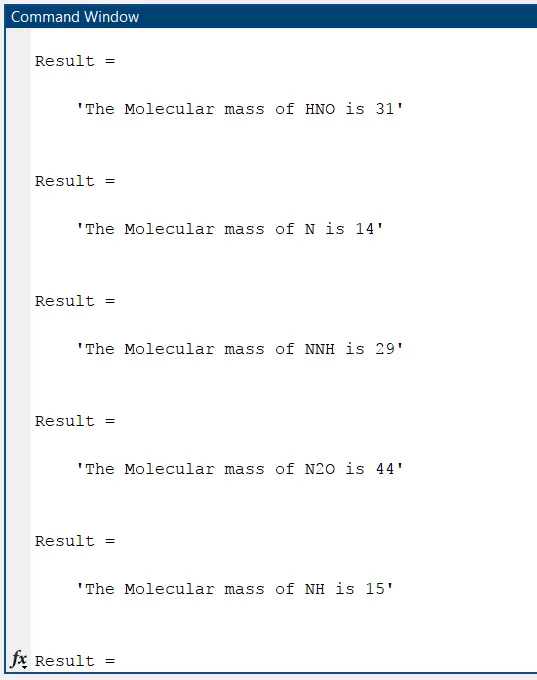
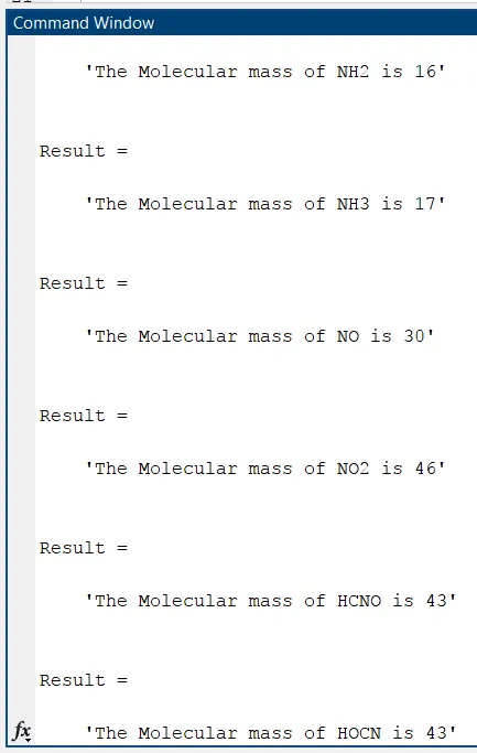
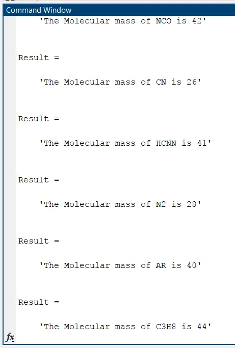
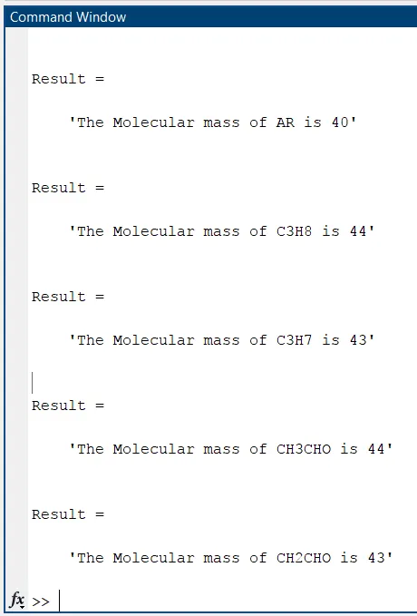
• Calculate the Molecular Mass of each element and display it in the command window.
• Plot the Temperature vs Enthalpy, Entropy, and Specific heat for all the elements.
• Dump each of the plots automatically in separate folders with the name of the element.

Procedure:

Data parsing is a method where one string of data gets converted into a different type of data. So let’s say you receive your data in raw HTML, a parser will take the said HTML and transform it into a more readable data format that can be easily read and understood. Parsing is necessary because different entities need the data to be in different forms. Parsing allows transforming data in a way that can be understood by specific software.

We will start by loading the Data file into the Matlab Program, So we should first check the format of the Data that we have and make sure the alignment is correct inside the file.

clear all
close all
clc

%Step-1 Loading Data
N1=fopen('THERMO.dat','r');
fgetl(N1); %To skip the first line Thermo
R=8.3145; %Universal Gas constant

So after loading the data we need to skip the header file so we will be using the 'fgetl' here. We will be placing the file under the name "N1" in our code. Each time we use the 'fgetl' the command reads the line automatically. So if we use fgetl twice we will be reading the second line.

Next, we need to capture the Global Temperature.

G_Temp=str2num(fgetl(N1));
GLT=G_Temp(1); % Global Low Temperature
GMT=G_Temp(2); % Global Mid  Temperature
GHT=G_Temp(3); % Global High Temperature 

So the global temperatures are in the Second line so Since we are using "fgetl" the second time it will read the Temperatures as Strings. So we convert it into a Number using str2num and separate the Global High, Low and Mid.

You can see that the second line only has the Global Temperatures so the above process will capture the Global Temperatures. So after that, we need to skip the remaining three line which is comments.

%Skipping the next three lines that contain comments!!
for z=1:3
    fgetl(N1);
end

Using the for loop we will be omitted the comment lines the loop will run for three lines hence skipping them.

while true

%Capturing the Element Name
line1=fgetl(N1);
if line1=="END"
    break
end

We will be starting to capture the remaining values so in order to make the code shorter we will be finding the values for one element and will be using a while loop with a condition to break the loop when we encounter the "END" at the end of the file.

We can use a for loop but for loop can be used only when we know the number of times the loop needs to run so a while loop will be more appropriate making the code universal.

There are four Lines in the above data. So we will be reading them as Line1, Line2, Line3, and Line4 using fgetl command.

Element=strtok(line1);
Local_Temp=strsplit(line1,' ' );%Splitting the local Temperature Line
Local_MT=str2num(Local_Temp{end-1});%Local Mid Temperature
Local_HT=str2num(Local_Temp{end-2});%Local High Temperature
Local_LT=str2num(Local_Temp{end-3});%Local Low Temperature
T_Avg=linspace(Local_LT,Local_HT,200);

We can see that the first Letter from Line1 is the element so we will be using 'strtok' which ignores the whitespaces and captures the first Letter or word. After that, we will be using strsplit to split the whitespaces in the Line1 so that we can capture the Temperatures separately. Then we will be using str2num and capture the Local temperatures.

The average temperature will be the range from Local to high temperature using linspace.

%Capturing the Coefficients
line2=fgetl(N1);
line3=fgetl(N1);
line4=fgetl(N1);

%Capturing the position of E in the Line2,3 and 4.
X=strfind(line2,'E');
Y=strfind(line3,'E');
Z=strfind(line4,'E');

So in order to capture the coefficients, we need to find the position of "E", So we will be using the strfind command. Here the X, Y, and Z variables now contain the position of E in lines line2,line3, and line 4.

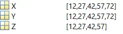
You can see that there are 5 "E's" in line2 and line3 and 4 in line4.

%Capturing Higher Temp coefficients
a1=str2num(line2(1:X(1)+3));
a2=str2num(line2(X(1)+4:X(2)+3));
a3=str2num(line2(X(2)+4:X(3)+3));
a4=str2num(line2(X(3)+4:X(4)+3));
a5=str2num(line2(X(4)+4:X(5)+3));
a6=str2num(line3(1:Y(1)+3));
a7=str2num(line3(Y(1)+4:Y(2)+3));

%Capturing Lower Temp coefficients
b1=str2num(line3(Y(2)+4:Y(3)+3));
b2=str2num(line3(Y(3)+4:Y(4)+3));
b3=str2num(line3(Y(4)+4:Y(5)+3));
b4=str2num(line4(1:Z(1)+3));
b5=str2num(line4(Z(1)+4:Z(2)+3));
b6=str2num(line4(Z(2)+4:Z(3)+3));
b7=str2num(line4(Z(3)+4:Z(4)+3));

The First 7 (a1 to a2)are high temperature and the second 7(b1 to b6)are low-temperature coefficients. With the position of "E", we will be calculating the coefficients and will be using str2num to convert the string to a number.

Since we have found the Coefficients we will be calculating the Enthalpy, Entropy, and Specific heat using the given Formula.

In order to make the code more simple we will be giving the formula as a function. below is the function for the formulas

function [H,Cp,S]=Thermodynamic(a1,a2,a3,a4,a5,a6,a7,b1,b2,b3,b4,b5,b6,b7,R,T_Avg,Local_MT);
for i=1:length(T_Avg)
    if T_Avg(i)>Local_MT
        H(i)= R*T_Avg(i)*(a1+a2*(T_Avg(i)/2)+a3*(T_Avg(i)^2/3)+a4*(T_Avg(i)^3/4)+a5*(T_Avg(i)^4/5)+a6/T_Avg(i));
        Cp(i)=R*(a1+a2*T_Avg(i)+a3*T_Avg(i)^2+a4*T_Avg(i)^3+a5*T_Avg(i)^4);
        S(i)=R*(a1*log(T_Avg(i))+a2*T_Avg(i)+a3*(T_Avg(i)^2/2)+a4*(T_Avg(i)^3/3)+a5*(T_Avg(i)^4/4)+a7);
        else
        H(i)= R*T_Avg(i)*(b1+b2*(T_Avg(i)/2)+b3*(T_Avg(i)^2/3)+b4*(T_Avg(i)^3/4)+b5*(T_Avg(i)^4/5)+b6/T_Avg(i));
        Cp(i)=R*(b1+b2*T_Avg(i)+b3*T_Avg(i)^2+b4*T_Avg(i)^3+b5*T_Avg(i)^4);
        S(i)=R*(b1*log(T_Avg(i))+b2*T_Avg(i)+b3*(T_Avg(i)^2/2)+b4*(T_Avg(i)^3/3)+b5*(T_Avg(i)^4/4)+b7);
       
    end
end
end

So we will be calculating the enthalpy, entropy, and Specific heat using a single function. The for loop is used so that we can calculate the values for the range of "T_Avg".

So the value of T_Avg will range from Local low to local high temperature. For the local low temperatures, the low coefficients(b1 to b7) must be used for the local high temperatures high coefficients(a1 to a7) must be used. So we will be using an "If" condition here so that if the T_Avg is less than Local_MT the Low coefficients will be used to calculate the values the high coefficients will be skipped. Hence if the T_Avg>Local_MT the High coefficients will be used.

You can see below how we are calling the Function for the Enthalpy, Entropy, and Specific heat.

%Calculating Enthalpy,Entropy and Specific Heat
[H,Cp,S]=Thermodynamic(a1,a2,a3,a4,a5,a6,a7,b1,b2,b3,b4,b5,b6,b7,R,T_Avg,Local_MT);

The next step is the plotting of the Enthalpy, Entropy, and Specific heat vs Temperature and for each element, the plot should be stored in a separate folder with the name of the element.

mkdir('C:UsersStudent-62DocumentsMATLABAnirudhAll Elements',Element);

The mkdir will create a Folder in the given directory and the name of the folder is a variable which is "Element" in our case. So for each loop new folder with the name of the element will be created.

The Next step is to plot all the Curves for Enthalpy,Entropy and Specific heat Vs Temperature for all the Elements.

figure(1)
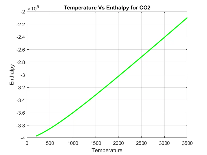
plot(T_Avg,H,'linewidth',2,'color','g')
title(sprintf('Temperature Vs Enthalpy for %s',Element))
xlabel('Temperature')
ylabel('Enthalpy')
grid on

figure(2)
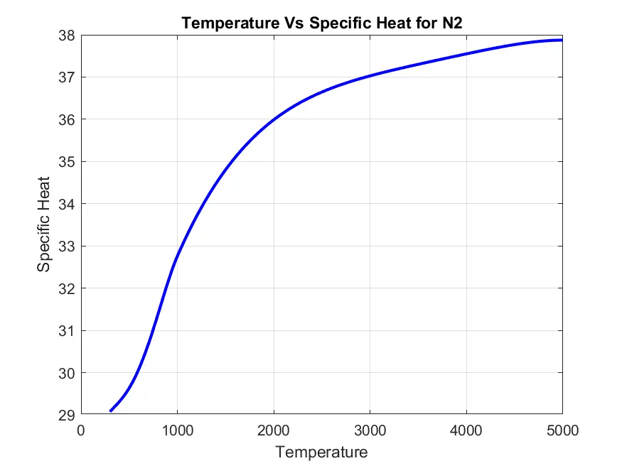
plot(T_Avg,Cp,'linewidth',2,'color','b')
title(sprintf('Temperature Vs Specific Heat for %s',Element))
xlabel('Temperature')
ylabel('Specific Heat')
grid on

figure(3)
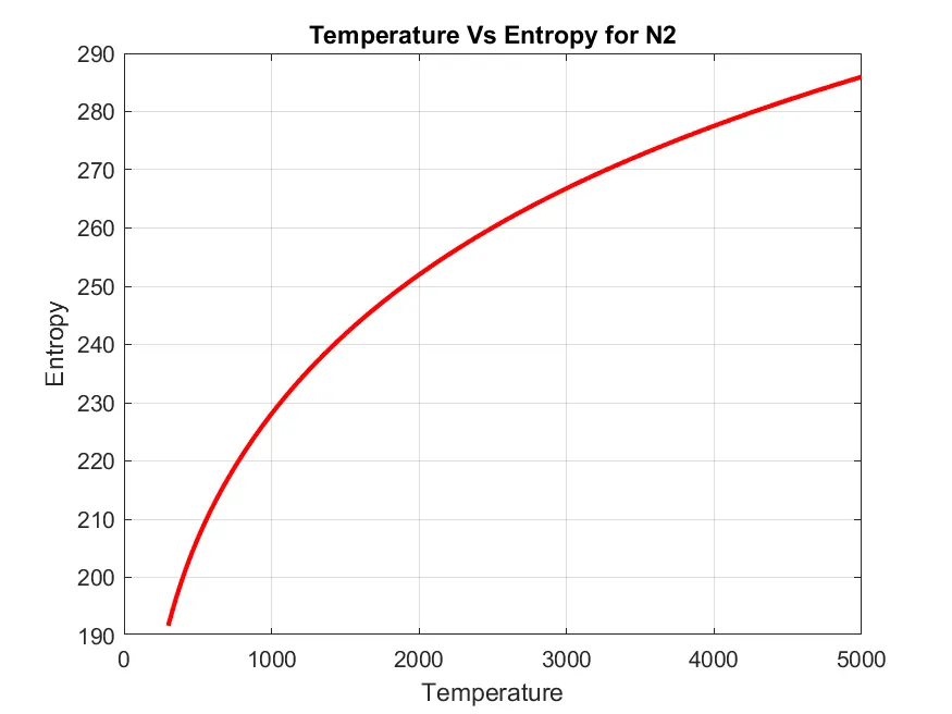
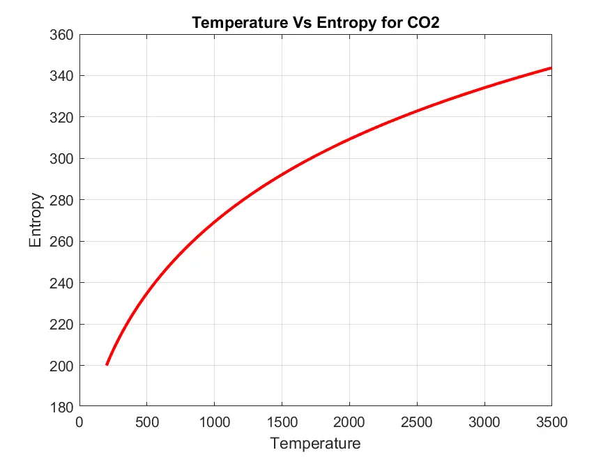
plot(T_Avg,S,'linewidth',2,'color','r')
title(sprintf('Temperature Vs Entropy for %s',Element))
xlabel('Temperature')
ylabel('Entropy')
grid on;

The Commands used are very similar to the commands we have used until now for plotting. We will just add a Sprintf to the title so that the name of the element will change for each loop in the title. All three graphs are represented in three different figures ie Figure(1), Figure(2), and Figure(3)

The next step is to save the Graphs into the file that we have created using the "mkdir" command.

cd(['C:UsersStudent-62DocumentsMATLABAnirudhAll Elements',Element])
saveas(1,'T_Vs_Enthalpy.png')
saveas(2,'T_Vs_Specific_Heat.png')
saveas(3,'T_Vs_Entropy.png')
oldFolder=cd('C:UsersStudent-62DocumentsMATLABAnirudh');

In order to save the Graphs, we need to give the New Directory where we have created the Folder with the element name so we will be using the command cd here. The "saveas" command is used to save the Graphs (figure(1),figure(2),figure(3)). The old folder command is used to direct the code to the old directory as the directory will change when saving the graphs.

The calculation for the Molecular Weight is Below:

We will be providing the Molecular weight in a separate function as shown below.

function [MM]=Molecular_Mass(Element);
Atoms=['H','C','O','N','A'];
Atomic_Number=[1 12 16 14 40];
MM=0;
for i=1:length(Element);
    for j=1:length(Atoms);
        if strcmpi(Element(i),Atoms(j));
            MM=MM+Atomic_Number(j);
            position=j;
        end
    end
        n=str2num(Element(i));
    if n>1;
        MM=MM+Atomic_Number(position)*(n-1);
    end
    end

We must first specify the Molecule and their Molecular mass which we have provided as Atoms and Atomic Number. The Atoms (Molecules) here are Individuals that are given in the data. The MM=0 is given before the starting of the Loop.

To find the Molecular weight we use a nested for loop. The first loop will run for the length of the Element and the second one will run for the length of Atoms. The if the loop is used with "strcmp" so that only if the Letter of both Element and Atom match the condition will be satisfied the molecular weight assigned to that letter will be calculated. The position command will capture the location of the letter in the Atoms Array.

The Nested loops won't be able to calculate the MM in Elements(N2), As it will calculate the first character N but won't capture the 2, This is when the (if n>1) condition will come and will include the 2 and adding it with the previously calculated MM using the previously assigned position and MM. Hence calculated the Molecular weight of the Element.

MM=Molecular_Mass(Element);
Result=sprintf('The Molecular Weight of %s is %d',Element,MM)

Here we are calling the previously created function into the main code so that we can display the Molecular weight of all the Elements. So the result will provide the Molecular weight of each element in the command window.

Please find the complete code below.

clear all
close all
clc

%Step-1 Loading Data
N1=fopen('THERMO.dat','r');
fgetl(N1); %To skip the first line Thermo
R=8.3145; %Universal Gas constant

G_Temp=str2num(fgetl(N1));
GLT=G_Temp(1); % Global Low Temperature
GMT=G_Temp(2); % Global Mid  Temperature
GHT=G_Temp(3); % Global High Temperature 

%Skipping the next three lines that contain comments!!
for K=1:3
    fgetl(N1);
end

while true

%Capturing the Element Name
line1=fgetl(N1);
if line1=="END"
    break
end

Element=strtok(line1);
Local_Temp=strsplit(line1,' ' );%Splitting the local Temperature Line
Local_MT=str2num(Local_Temp{end-1});%Local Mid Temperature
Local_HT=str2num(Local_Temp{end-2});%Local High Temperature
Local_LT=str2num(Local_Temp{end-3});%Local Low Temperature
T_Avg=linspace(Local_LT,Local_HT,200);

%Capturing the Coefficients
line2=fgetl(N1);
line3=fgetl(N1);
line4=fgetl(N1);

%Capturing the position of E in the Line2,3 and 4.
X=strfind(line2,'E');
Y=strfind(line3,'E');
Z=strfind(line4,'E');

%Capturing Higher Temp coefficients
a1=str2num(line2(1:X(1)+3));
a2=str2num(line2(X(1)+4:X(2)+3));
a3=str2num(line2(X(2)+4:X(3)+3));
a4=str2num(line2(X(3)+4:X(4)+3));
a5=str2num(line2(X(4)+4:X(5)+3));
a6=str2num(line3(1:Y(1)+3));
a7=str2num(line3(Y(1)+4:Y(2)+3));

%Capturing Lower Temp coefficients

b1=str2num(line3(Y(2)+4:Y(3)+3));
b2=str2num(line3(Y(3)+4:Y(4)+3));
b3=str2num(line3(Y(4)+4:Y(5)+3));
b4=str2num(line4(1:Z(1)+3));
b5=str2num(line4(Z(1)+4:Z(2)+3));
b6=str2num(line4(Z(2)+4:Z(3)+3));
b7=str2num(line4(Z(3)+4:Z(4)+3));

%Calculating Enthalpy,Entropy and Specific Heat
[H,Cp,S]=Thermodynamic(a1,a2,a3,a4,a5,a6,a7,b1,b2,b3,b4,b5,b6,b7,R,T_Avg,Local_MT);

%Saving the Elements in the Given Directory in new 
mkdir('C:UsersStudent-62DocumentsMATLABAnirudhAll Elements',Element);

figure(1)
plot(T_Avg,H,'linewidth',2,'color','g')
title(sprintf('Temperature Vs Enthalpy for %s',Element))
xlabel('Temperature')
ylabel('Enthalpy')
grid on

figure(2)
plot(T_Avg,Cp,'linewidth',2,'color','b')
title(sprintf('Temperature Vs Specific Heat for %s',Element))
xlabel('Temperature')
ylabel('Specific Heat')
grid on

figure(3)
plot(T_Avg,S,'linewidth',2,'color','r')
title(sprintf('Temperature Vs Entropy for %s',Element))
xlabel('Temperature')
ylabel('Entropy')
grid on;

cd(['C:UsersStudent-62DocumentsMATLABAnirudhAll Elements',Element])
saveas(1,'T_Vs_Enthalpy.png')
saveas(2,'T_Vs_Specific_Heat.png')
saveas(3,'T_Vs_Entropy.png')
oldFolder=cd('C:UsersStudent-62DocumentsMATLABAnirudh');

MM=Molecular_Mass(Element);
Result=sprintf('The Molecular Weight of %s is %d',Element,MM)

end

Result Images:

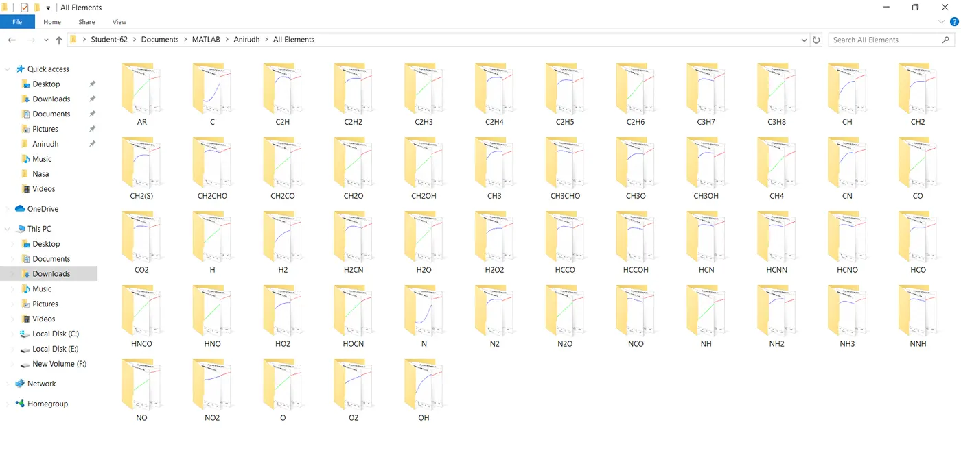
The below image shows how individual folders are created for each element and their Graphs have been saved in those folders.

Molecular Weight:

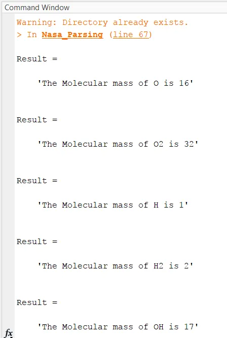
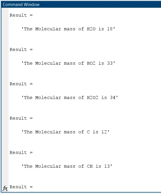
The below images show the Molecular weight in the command window

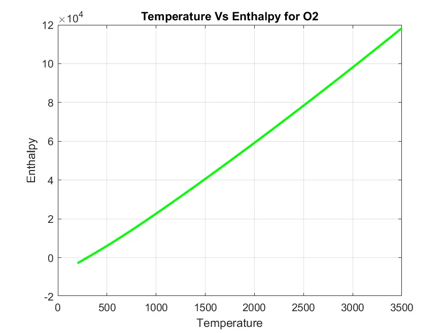
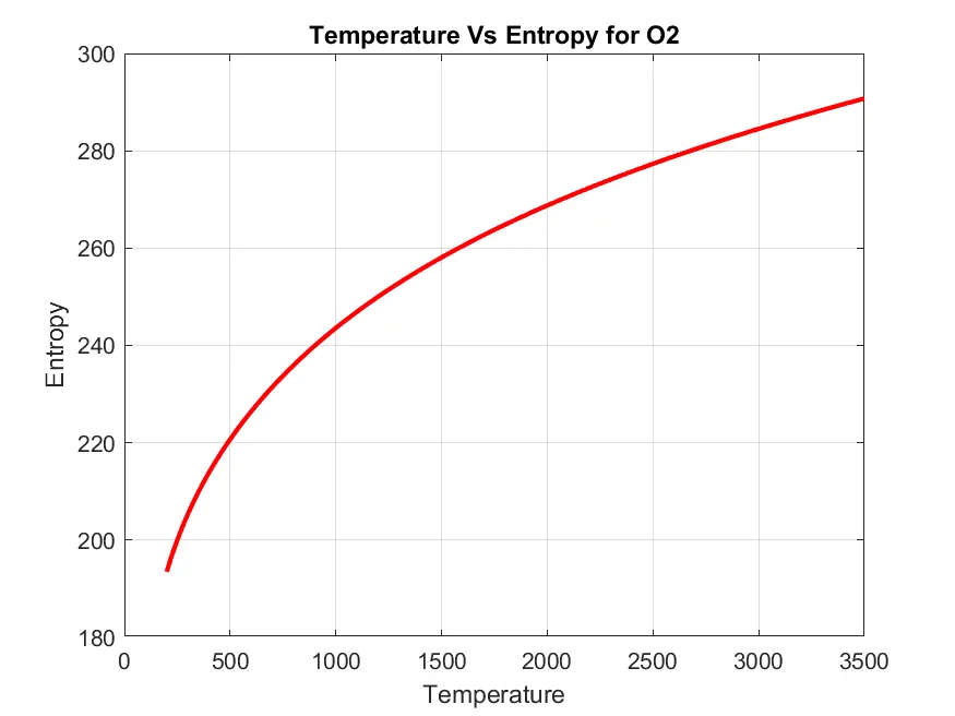
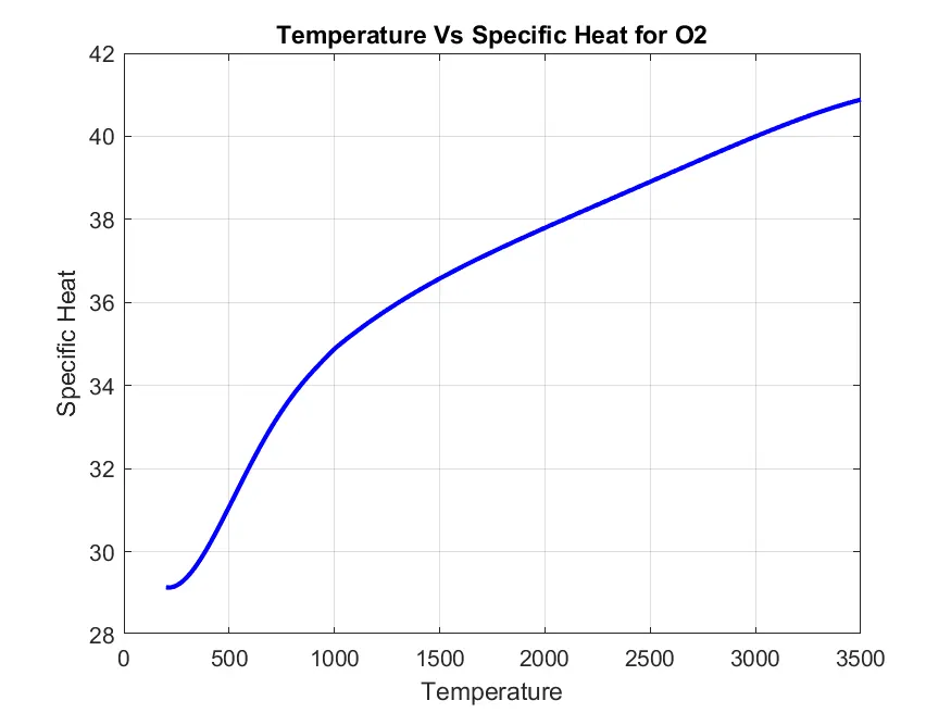
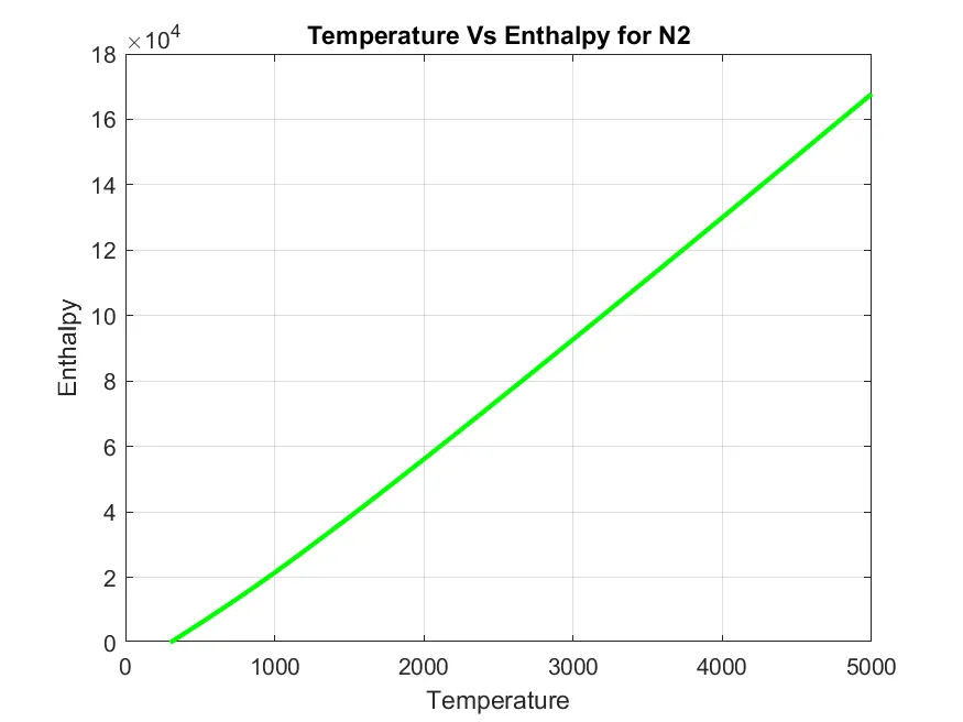
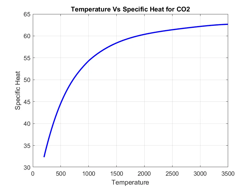
Plots of 02,N2, and CO2:

The graph of Enthalpy, Entropy, and Specific heat Vs Temperature is below:

For O2:

For N2:

For Co2:

Below is the link for the rest of the Graphs:

https://drive.google.com/file/d/12PrgWDGDDIjULMPfNSMur9gW214dtc_q/view?usp=sharing

Conclusion:

From the given Nasa data we have separated the coefficients and calculated the Enthalpy, Entropy, and Specific heat for the Species and plotted the Graphs, and saved them in separate folders.