Challenge

Project 1 - Parsing NASA thermodynamic data

AAksharat Jain27 Apr 2024

Aim:

The aim of this project is to develop a software tool that can effectively parse NASA thermodynamic data files, extract necessary coefficients, and utilize them to calculate thermodynamic properties for various chemical species. This tool should be capable of handling the complexity and volume of the data provided by NASA, enabling researchers and engineers to access and utilize thermodynamic information efficiently. Additionally, the software should automate the process of generating plots for specific heat (Cp), enthalpy (H), and entropy (S) for each species within their unique temperature ranges, facilitating further analysis and visualization of thermodynamic data.

Objective:

Coefficient Extraction and Calculation: Develop algorithms to parse the NASA thermodynamic data file and extract the polynomial coefficients for each chemical species. Utilize these coefficients to calculate thermodynamic properties within their respective temperature ranges.
Molecular Weight Calculation: Implement methods to determine the molecular weight of each chemical species based on their constituent elements, aiding in further analysis and comparison.
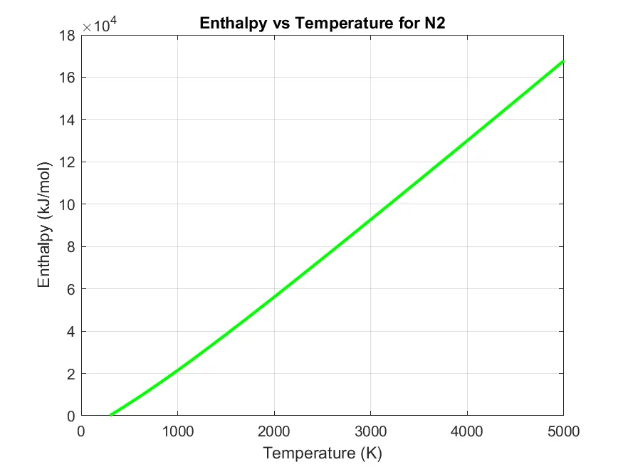
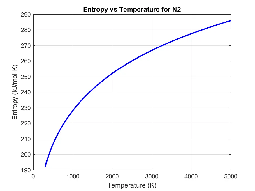
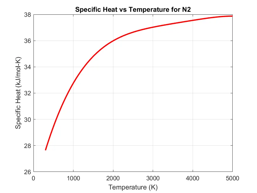
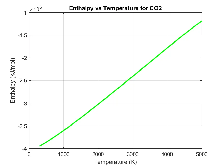
Property Plotting: Create algorithms to plot the thermodynamic properties (Cp, H, S) against temperature for each chemical species using the extracted coefficients. These plots will provide insights into the variation of properties with temperature.
Automated File Management: Develop mechanisms to automatically save the generated plots as images and organize them into separate folders for each species. This ensures efficient management and retrieval of the parsed data and results.
Integration and User Interface: Integrate all parsing and analysis functionalities into a user-friendly program. Design the interface to accept the NASA thermodynamic data file as input and output the parsed coefficients and plotted properties.
Documentation and Report Writing: Document the parsing algorithms, coefficient extraction methods, property calculation procedures, and plotting techniques in detail. Write a comprehensive report outlining the objectives, methodology, results, and conclusions of the project.

Problem Statement:

NASA provides extensive thermodynamic data in the form of polynomial equations and coefficients for numerous chemical species. However, accessing and utilizing this data effectively presents several challenges:

Accurate extraction of polynomial coefficients from the provided data file.
Efficient calculation of thermodynamic properties using the extracted coefficients.
Determination of the molecular weight of each chemical species for comparative analysis.
Visualization of thermodynamic property variations with temperature through plotting.
Automation of file management to organize and store the parsed data and results effectively.

This project aims to address these challenges by developing a computational tool capable of parsing NASA thermodynamic data, extracting coefficients, calculating properties, plotting results, and managing files automatically.

Theories Related to the Question:

Thermodynamic Properties: Thermodynamic properties describe the behavior of chemical species in relation to energy and temperature. Enthalpy (H), entropy (S), and specific heat (Cp) are fundamental properties used to characterize the thermodynamic state of a substance.
NASA Polynomial Equations: NASA has developed polynomial equations to represent thermodynamic properties for various chemical species. These equations typically involve coefficients that are specific to each species and temperature range, allowing accurate calculation of thermodynamic properties over a wide range of conditions.
Molecular Weight Calculation: The molecular weight of a chemical species is determined by summing the atomic weights of its constituent atoms. This value is crucial for various thermodynamic calculations and serves as a basis for understanding the behavior of chemical compounds.
Temperature Dependency of Thermodynamic Properties: Thermodynamic properties such as Cp, H, and S exhibit temperature dependency, meaning their values change with variations in temperature. Understanding this dependency is essential for predicting and analyzing the behavior of chemical species under different temperature conditions.

By addressing these theories and objectives, the software tool developed in this project will provide researchers and engineers with a valuable resource for accessing, analyzing, and visualizing NASA thermodynamic data effectively.

File Parsing:

File parsing is the process of systematically analyzing the contents of a file, typically in a structured or semi-structured format, to extract relevant information according to predefined rules or patterns. This process involves reading the data from the file, interpreting its structure, and converting it into a format that can be processed or analyzed by a computer program.

In this context, parsing NASA's thermodynamic data files, like THERMO.dat, is essential for extracting coefficients used to evaluate thermodynamic properties of chemical species. These coefficients enable modeling complex phenomena like chemical reactions and combustion. Parsing involves reading the file, extracting coefficients, and considering species-specific temperature ranges for accurate analysis. Beyond coefficients, parsing also involves calculating molecular weights and generating plots to visualize thermodynamic properties. Through efficient parsing, researchers and engineers gain insights into the behavior of chemical species under various conditions, aiding in scientific understanding and engineering design. Overall, file parsing in this scenario is fundamental for extracting crucial information from thermodynamic data files, facilitating the development of accurate models and simulations for diverse applications.

NASA Thermodynamic File:

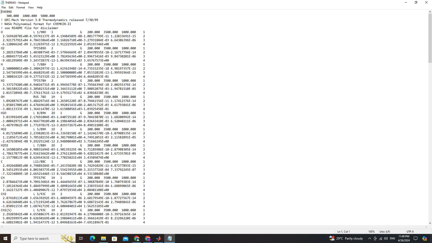
A NASA Thermodynamic File, typically with a .dat extension, stores data used to calculate the thermodynamic properties of various substances at different temperatures. These files are crucial for researchers and engineers in fields like aerospace, combustion, and chemical processing.

The file contains a set of 14 coefficients for 53 each chemical species (molecule or atom). These coefficients are used in specific polynomial equations to determine a substance's:

Specific heat (Cp) - Ability to absorb heat
Enthalpy (H) - Total energy of a system
Entropy (S) - Measure of randomness or disorder

NASA Thermodynamic Polynomial:

Enthalpy (H):

Enthalpy represents the total energy of a thermodynamic system, including its internal energy and the pressure-volume work term. It's a state function, meaning its value depends only on the state of the system (temperature, pressure, etc.) and not on the path taken to reach that state.

Imagine a system like a compressed gas in a cylinder. The internal energy of the gas represents the random motion of its molecules. Enthalpy takes into account not just this internal energy but also the work done by the gas when its volume changes against the external pressure (e.g., the pressure exerted by the piston in the cylinder).

Units: Enthalpy is typically measured in Joules (J) or kilojoules (kJ) in scientific applications.

Entropy (S):

Entropy is a measure of the disorder or randomness within a thermodynamic system. A higher entropy state signifies a more disordered system. Entropy is also a state function.

Think of entropy as a measure of how spread out the energy is in a system. A system with all its energy concentrated in a specific way (highly ordered) would have low entropy. Conversely, a system where the energy is evenly distributed among its various components in a more chaotic manner would have high entropy.

Units: Entropy is typically measured in joules per kelvin (J/K) or kilojoules per kelvin (kJ/K).

Specific Heat (Cp):

Specific heat capacity (Cp) is a property of a material that indicates the amount of heat energy required to raise the temperature of 1 gram of that material by 1 degree Celsius (or Kelvin) at constant pressure. It essentially tells you how much heat a material can store per unit mass for a specific temperature increase.

Imagine heating water and milk. Water has a higher specific heat than milk. This means it takes more heat energy to raise the temperature of 1 gram of water by 1 degree Celsius compared to 1 gram of milk under the same pressure conditions.

Units: Specific heat is typically measured in joules per gram per kelvin (J/g/K) or kilojoules per gram per kelvin (kJ/g/K).

Molecular Weight:

Molecular weight, also known as molecular mass or molar mass, is a fundamental property of a substance in chemistry. It represents the mass of a molecule relative to the unified atomic mass unit (amu) and is expressed in grams per mole (g/mol).

In simpler terms, molecular weight tells us how much one mole of a substance weighs. A mole is a unit used in chemistry to represent a specific number of atoms or molecules, just like a dozen represents 12 items. One mole of any substance contains Avogadro's number of molecules or atoms, which is approximately 6.022×10236.022×1023.

For example, the molecular weight of water (H₂O) is approximately 18.015 g/mol. This means that one mole of water molecules weighs about 18.015 grams. Similarly, the molecular weight of carbon dioxide (CO₂) is approximately 44.01 g/mol, indicating that one mole of carbon dioxide molecules weighs 44.01 grams.

Units: Molecular weight is typically expressed in grams per mole (g/mol).

Formulas:

The formulas given are the ones used by NASA to evaluate thermodynamic properties of various chemical species. They are in the form of a high-temperature polynomial and and and low-temperature polynomial to capture the behavior of a material’s properties across a wider range of temperatures.

Here’s a breakdown of the formulas:

High-Temperature:
- Specific Heat Capacity (Cp/R): Cp/R = a1 + a2T + a3T^2 + a4T^3 + a5T^4 + a6*T^5 + a7/T (Eq. 1)
- Enthalpy (H/RT): H/RT = a1 + a2T/2 + a3T^2/3 + a4T^3/4 + a5T^5/5 + a6/T + a7*T (Eq. 2)

Low-Temperature:
- Specific Heat Capacity (Cp/R): Cp/R = a8 + a9T + a10T^2 + a11T^3 + a12T^4 + a13*T^5 + a14/T (Eq. 3)
- Enthalpy (H/RT): H/RT = a8 + a9T/2 + a10T^2/3 + a11T^3/4 + a12T^5/5 + a13/T + a14*T (Eq. 4)

Entropy (valid for all temperatures):
- S/R = a1ln(T) + a2T + a3T^2/2 + a4T^3/3 + a5*T^4/4 + a6 (Eq. 5)

where:

Cp is the specific heat at constant pressure
R is the universal gas constant
T is the temperature
a1, a2, a3, etc. are the coefficients

Key Points:

There are a total of 14 coefficients (a1 to a14) used in the NASA thermodynamic data.
The first 7 coefficients (a1 to a7) are used in the high-temperature formulas (Eq. 1 & Eq. 2).
The second 7 coefficients (a8 to a14) are used in the low-temperature formulas (Eq. 3 & Eq. 4).
The entropy formula (Eq. 5) uses only the first 6 coefficients (a1 to a6) and is valid across all temperatures.

Commands Used:

clear all: This command clears all variables from the workspace.
close all: This command closes all open figures.
clc: This command clears the command window.
mkdir: This command creates a new directory (folder) with the specified name.
fopen: This command opens a file specified by its filename and returns a file identifier.
fclose: This command closes the file associated with the specified file identifier.
fgetl: This command reads a line from a file and advances the file pointer to the next line.
strsplit: This command splits a string into substrings based on a specified delimiter and returns the substrings as elements of a cell array.
str2double: This command converts a string to a double-precision floating-point number.
linspace: This command generates linearly spaced vector of points between specified start and end points.
fprintf: This command writes formatted data to a file or the command window.
fullfile: This command constructs a full filename from directory and file name parts.
mkdir: This command creates a new directory.
fid: This is a file identifier returned by fopen when opening a file.
xlabel: This command sets the label for the x-axis in a plot.
ylabel: This command sets the label for the y-axis in a plot.
title: This command sets the title for a plot.
plot: This command generates a 2D plot of the data provided.
grid on: This command displays the grid lines on a plot.
saveas: This command saves a figure to a file with the specified filename.
close: This command closes the current figure.

Matlab Program:

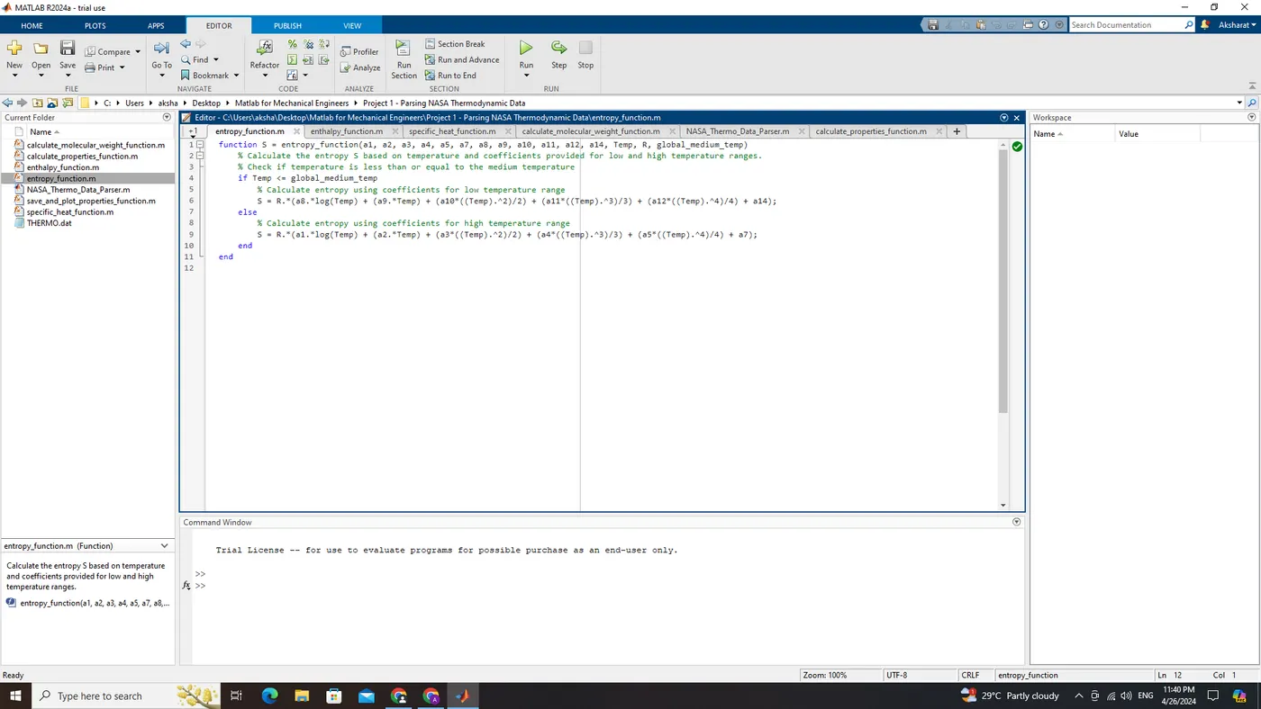
entropy_function

function S = entropy_function(a1, a2, a3, a4, a5, a7, a8, a9, a10, a11, a12, a14, Temp, R, global_medium_temp)
    % Calculate the entropy S based on temperature and coefficients provided for low and high temperature ranges.
    % Check if temperature is less than or equal to the medium temperature
    if Temp <= global_medium_temp
        % Calculate entropy using coefficients for low temperature range
        S = R.*(a8.*log(Temp) + (a9.*Temp) + (a10*((Temp).^2)/2) + (a11*((Temp).^3)/3) + (a12*((Temp).^4)/4) + a14);
    else
        % Calculate entropy using coefficients for high temperature range
        S = R.*(a1.*log(Temp) + (a2.*Temp) + (a3*((Temp).^2)/2) + (a4*((Temp).^3)/3) + (a5*((Temp).^4)/4) + a7);
    end
end

Explanation:

Function Definition

function S = entropy_function(a1, a2, a3, a4, a5, a7, a8, a9, a10, a11, a12, a14, Temp, R, global_medium_temp)

This defines a MATLAB function named entropy_function with input arguments a1 through a14, Temp, R, and global_medium_temp, and an output argument S.

Function Description

% Calculate the entropy S based on temperature and coefficients provided for low and high temperature ranges.

This comment describes the purpose of the function, which is to calculate the entropy (S) based on temperature (Temp) and coefficients provided for both low and high temperature ranges.

Entropy Calculation

    if Temp <= global_medium_temp
        S = R.*(a8.*log(Temp) + (a9.*Temp) + (a10*((Temp).^2)/2) + (a11*((Temp).^3)/3) + (a12*((Temp).^4)/4) + a14);
    else
        S = R.*(a1.*log(Temp) + (a2.*Temp) + (a3*((Temp).^2)/2) + (a4*((Temp).^3)/3) + (a5*((Temp).^4)/4) + a7);
    end

This part of the code checks if the input temperature Temp is less than or equal to the medium temperature global_medium_temp. Depending on the result, it calculates the entropy S using different sets of coefficients (a1 through a14). If the temperature is less than or equal to the medium temperature, it uses coefficients for the low temperature range; otherwise, it uses coefficients for the high temperature range.

The entropy is calculated using the standard formula:

`S_(low) = R * (a_8 * ln(Temp) + a_9 * Temp + (a_10 * (Temp)^2)/2 + (a_11 * (Temp)^3)/3 + (a_12 * (Temp)^4)/4 +a_14)`

`S_(high) = R * (a_1 * ln(Temp) + a_2 * Temp + (a_3 * (Temp)^2)/2 + (a_4 * (Temp)^3)/3 + (a_5 * (Temp)^4)/4 +a_7)`

where R is the universal gas constant, and a1 through a5 and a7 are coefficients.

Function Output

end

This marks the end of the function definition.

Overall, this function calculates the entropy based on temperature and coefficients provided for both low and high temperature ranges. It follows a conditional logic to select the appropriate set of coefficients for calculation.

////

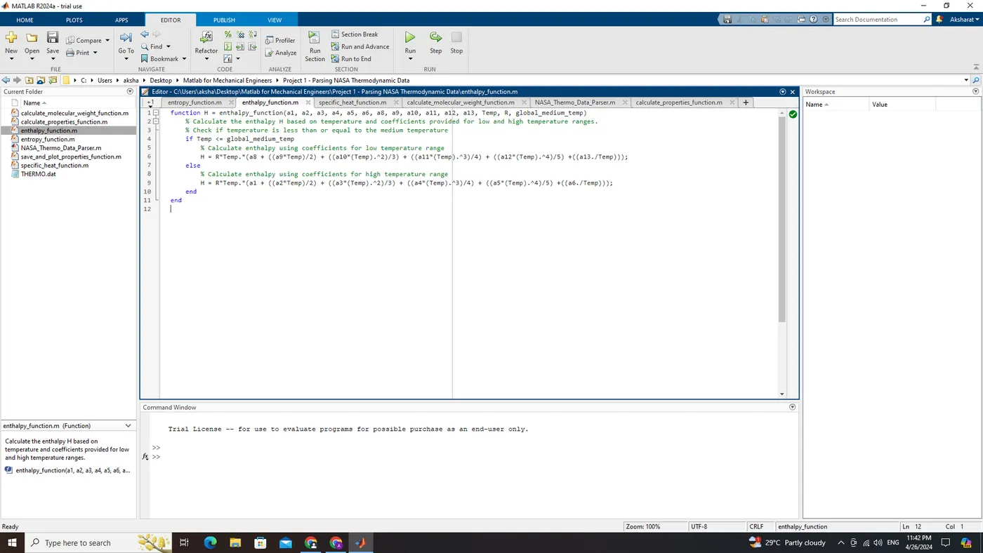
enthalpy_function

function H = enthalpy_function(a1, a2, a3, a4, a5, a6, a8, a9, a10, a11, a12, a13, Temp, R, global_medium_temp)
    % Calculate the enthalpy H based on temperature and coefficients provided for low and high temperature ranges.
    % Check if temperature is less than or equal to the medium temperature
    if Temp <= global_medium_temp
        % Calculate enthalpy using coefficients for low temperature range
        H = R*Temp.*(a8 + ((a9*Temp)/2) + ((a10*(Temp).^2)/3) + ((a11*(Temp).^3)/4) + ((a12*(Temp).^4)/5) +((a13./Temp)));
    else
        % Calculate enthalpy using coefficients for high temperature range
        H = R*Temp.*(a1 + ((a2*Temp)/2) + ((a3*(Temp).^2)/3) + ((a4*(Temp).^3)/4) + ((a5*(Temp).^4)/5) +((a6./Temp)));
    end
end

Explanation:

Function Defintion

function H = enthalpy_function(a1, a2, a3, a4, a5, a6, a8, a9, a10, a11, a12, a13, Temp, R, global_medium_temp)

This defines a MATLAB function named enthalpy_function with input arguments a1 through a13, Temp, R, and global_medium_temp, and an output argument H.

Function Description

% Calculate the enthalpy H based on temperature and coefficients provided for low and high temperature ranges.

This comment describes the purpose of the function, which is to calculate the enthalpy (H) based on temperature (Temp) and coefficients provided for both low and high temperature ranges.

Enthalpy Calculation

    if Temp <= global_medium_temp
        H = R*Temp.*(a8 + ((a9*Temp)/2) + ((a10*(Temp).^2)/3) + ((a11*(Temp).^3)/4) + ((a12*(Temp).^4)/5) +((a13./Temp)));
    else
        H = R*Temp.*(a1 + ((a2*Temp)/2) + ((a3*(Temp).^2)/3) + ((a4*(Temp).^3)/4) + ((a5*(Temp).^4)/5) +((a6./Temp)));
    end

This part of the code checks if the input temperature Temp is less than or equal to the medium temperature global_medium_temp. Depending on the result, it calculates the enthalpy H using different sets of coefficients (a1 through a13). If the temperature is less than or equal to the medium temperature, it uses coefficients for the low temperature range; otherwise, it uses coefficients for the high temperature range.

The enthalpy is calculated using the standard formula:

`H_(low) = R * Temp * (a_8 + (a_9 * Temp)/2 + (a_10 * (Temp)^2)/3 + (a_11 * (Temp)^3)/4 + (a_12 * (Temp)^4)/5 + (a_13)/(Temp))`

`H_(high) = R * Temp * (a_1 + (a_2 * Temp)/2 + (a_3 * (Temp)^2)/3 + (a_4 * (Temp)^3)/4 + (a_5 * (Temp)^4)/5 + (a_6)/(Temp))`

where
R is the universal gas constant, and a1 through a6 anda8 through a13 are coefficients.

Function Output

end

This marks the end of the function definition.

Overall, this function calculates the enthalpy based on temperature and coefficients provided for both low and high temperature ranges. It follows a conditional logic to select the appropriate set of coefficients for calculation.

////

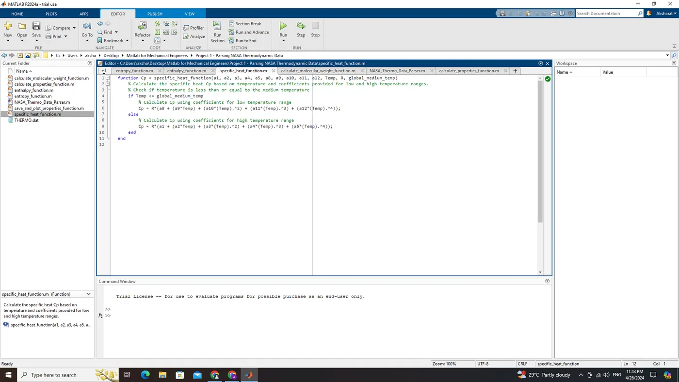
specific_heat_function

function Cp = specific_heat_function(a1, a2, a3, a4, a5, a8, a9, a10, a11, a12, Temp, R, global_medium_temp)
    % Calculate the specific heat Cp based on temperature and coefficients provided for low and high temperature ranges.
    % Check if temperature is less than or equal to the medium temperature
    if Temp <= global_medium_temp
        % Calculate Cp using coefficients for low temperature range
        Cp = R*(a8 + (a9*Temp) + (a10*(Temp).^2) + (a11*(Temp).^3) + (a12*(Temp).^4)); 
    else
        % Calculate Cp using coefficients for high temperature range
        Cp = R*(a1 + (a2*Temp) + (a3*(Temp).^2) + (a4*(Temp).^3) + (a5*(Temp).^4));
    end
end

Explanation:

Function Definition

function Cp = specific_heat_function(a1, a2, a3, a4, a5, a8, a9, a10, a11, a12, Temp, R, global_medium_temp)

This defines a MATLAB function named specific_heat_function with input arguments a1 through a12, Temp, R, and global_medium_temp, and an output argument Cp.

Function Description

% Calculate the specific heat Cp based on temperature and coefficients provided for low and high temperature ranges.

This comment describes the purpose of the function, which is to calculate the specific heat capacity at constant pressure (Cp) based on temperature (Temp) and coefficients provided for both low and high temperature ranges.

Specific Heat Calculation

    if Temp <= global_medium_temp
        Cp = R*(a8 + (a9*Temp) + (a10*(Temp).^2) + (a11*(Temp).^3) + (a12*(Temp).^4)); 
    else
        Cp = R*(a1 + (a2*Temp) + (a3*(Temp).^2) + (a4*(Temp).^3) + (a5*(Temp).^4));
    end

This part of the code checks if the input temperature Temp is less than or equal to the medium temperature global_medium_temp. Depending on the result, it calculates the specific heat capacity Cp using different sets of coefficients (a1 through a12). If the temperature is less than or equal to the medium temperature, it uses coefficients for the low temperature range; otherwise, it uses coefficients for the high temperature range.

The specific heat capacity is calculated using the standard formula:

`C_p(low) = R * (a_8 + a_9 * Temp + a_10 * (Temp)^2 + a_11 * (Temp)^3 + a_12 * (Temp)^4)`

`C_p(high) = R * (a_1 + a_2 * Temp + a_3 * (Temp)^2 + a_4 * (Temp)^3 + a_5 * (Temp)^4)`

where R is the universal gas constant, and a1 through a5 and a8 through a12 are coefficients.

Function Output

end

This marks the end of the function definition.

Overall, this function calculates the specific heat capacity at constant pressure (Cp) based on temperature and coefficients provided for both low and high temperature ranges. It follows a conditional logic to select the appropriate set of coefficients for calculation.

////

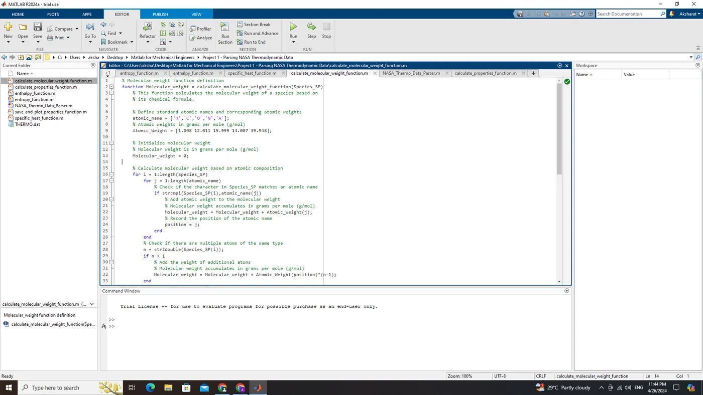
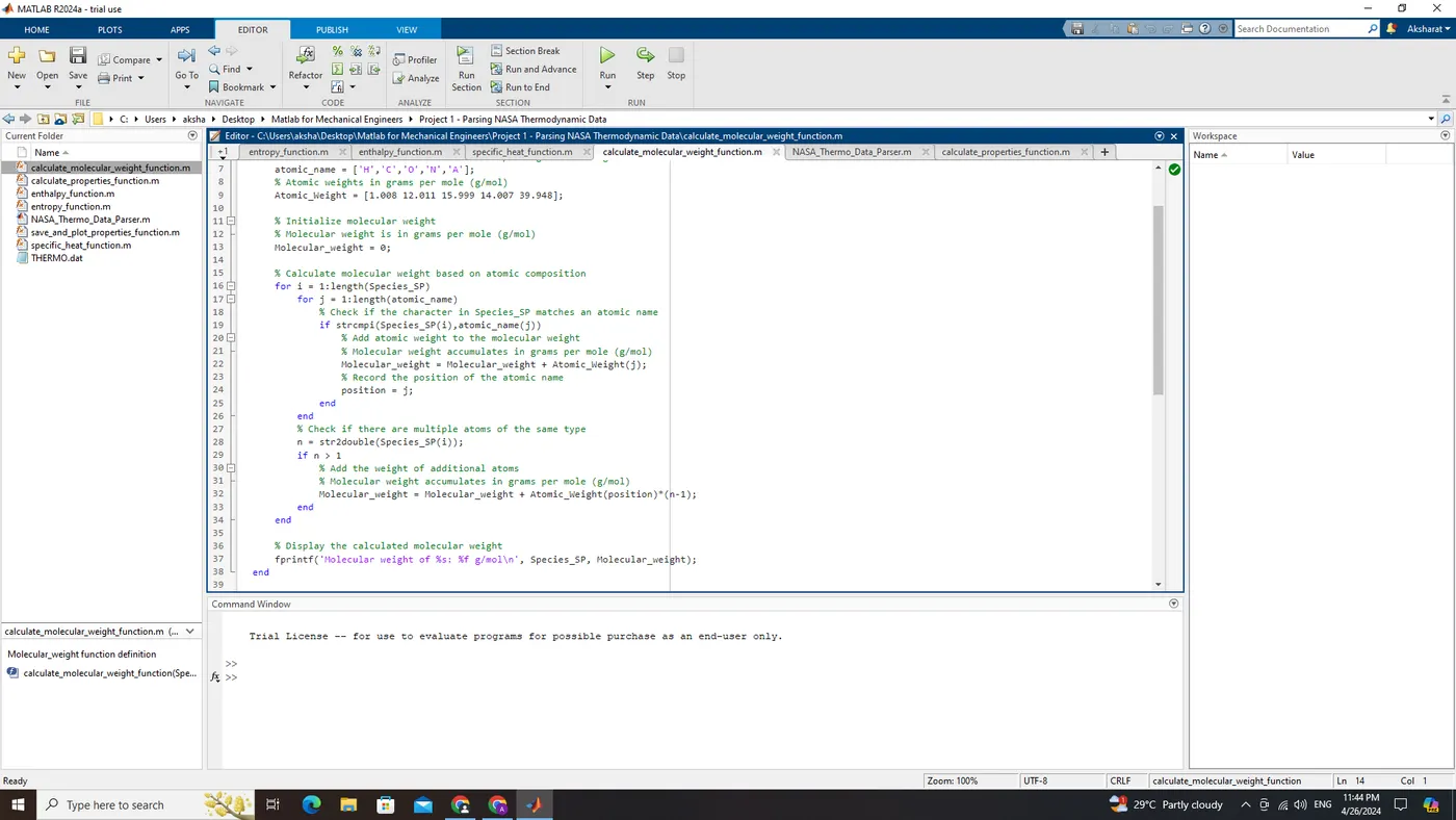
calculate_molecular_weight_function

% Molecular_weight function definition
function Molecular_weight = calculate_molecular_weight_function(Species_SP)
    % This function calculates the molecular weight of a species based on
    % its chemical formula.

    % Define standard atomic names and corresponding atomic weights
    atomic_name = ['H','C','O','N','A'];             
    % Atomic weights in grams per mole (g/mol)
    Atomic_Weight = [1.008 12.011 15.999 14.007 39.948];     

    % Initialize molecular weight
    % Molecular weight is in grams per mole (g/mol)
    Molecular_weight = 0;

    % Calculate molecular weight based on atomic composition
    for i = 1:length(Species_SP)
        for j = 1:length(atomic_name)
            % Check if the character in Species_SP matches an atomic name
            if strcmpi(Species_SP(i),atomic_name(j))
                % Add atomic weight to the molecular weight
                % Molecular weight accumulates in grams per mole (g/mol)
                Molecular_weight = Molecular_weight + Atomic_Weight(j);
                % Record the position of the atomic name
                position = j;
            end
        end
        % Check if there are multiple atoms of the same type
        n = str2double(Species_SP(i));
        if n > 1
            % Add the weight of additional atoms
            % Molecular weight accumulates in grams per mole (g/mol)
            Molecular_weight = Molecular_weight + Atomic_Weight(position)*(n-1);
        end
    end
    
    % Display the calculated molecular weight
    fprintf('Molecular weight of %s: %f g/mol\n', Species_SP, Molecular_weight);
end

Explanation:

Function Definition

function Molecular_weight = calculate_molecular_weight_function(Species_SP)

This defines a MATLAB function named calculate_molecular_weight_function with an input argument Species_SP representing the chemical formula of a species and an output argument Molecular_weight representing its molecular weight.

Function Description

% This function calculates the molecular weight of a species based on
% its chemical formula.

This comment describes the purpose of the function, which is to calculate the molecular weight of a species based on its chemical formula.

Atomic Names and Weights Initialization

    atomic_name = ['H','C','O','N','A'];             
    Atomic_Weight = [1.008 12.011 15.999 14.007 39.948];

This section initializes two arrays: atomic_name, which contains standard atomic names (e.g., 'H' for hydrogen, 'C' for carbon, etc.), and Atomic_Weight, which contains corresponding atomic weights in grams per mole (g/mol).

Molecular Weight Initialization

    Molecular_weight = 0;

This initializes the variable Molecular_weight to zero. It will accumulate the molecular weight of the species as the calculation proceeds.

Molecular Weight Calculation

    for i = 1:length(Species_SP)
        for j = 1:length(atomic_name)
            if strcmpi(Species_SP(i),atomic_name(j))
                Molecular_weight = Molecular_weight + Atomic_Weight(j);
                position = j;
            end
        end
        n = str2double(Species_SP(i));
        if n > 1
            Molecular_weight = Molecular_weight + Atomic_Weight(position)*(n-1);
        end
    end

This section iterates over each character in the input chemical formula Species_SP. For each character, it checks if it matches any of the standard atomic names (atomic_name). If a match is found, it adds the corresponding atomic weight (Atomic_Weight) to the Molecular_weight. If there are multiple atoms of the same type indicated by a numeric character (e.g., 'H2' for hydrogen), it adds the weight of additional atoms accordingly.

Displaying Calculated Molecular Weight

    fprintf('Molecular weight of %s: %f g/mol\n', Species_SP, Molecular_weight);

This section displays the calculated molecular weight of the species using fprintf.

Function Output

end

This marks the end of the function definition.

Overall, this function calculates the molecular weight of a species based on its chemical formula by iterating over the characters in the formula, matching them with standard atomic names, and summing up the corresponding atomic weights.

////

MAIN CODE

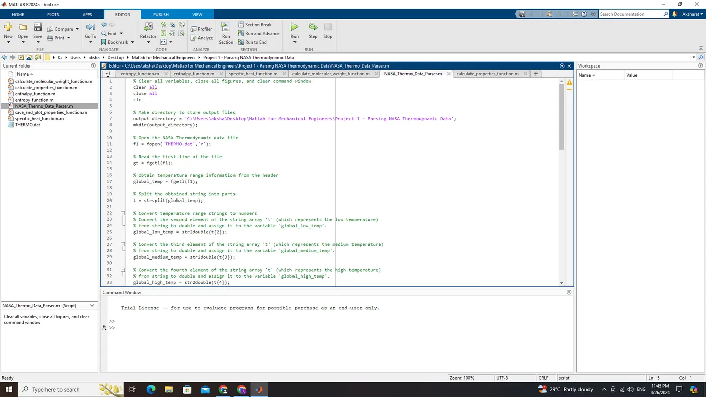
NASA_Thermo_Data_Parser

% Clear all variables, close all figures, and clear command window
clear all
close all
clc

% Make directory to store output files
output_directory = 'C:\Users\aksha\Desktop\Matlab for Mechanical Engineers\Project 1 - Parsing NASA Thermodynamic Data';
mkdir(output_directory);

% Open the NASA Thermodynamic data file
f1 = fopen('THERMO.dat','r');

% Read the first line of the file
gt = fgetl(f1);

% Obtain temperature range information from the header
global_temp = fgetl(f1);

% Split the obtained string into parts
t = strsplit(global_temp);

% Convert temperature range strings to numbers
% Convert the second element of the string array 't' (which represents the low temperature)
% from string to double and assign it to the variable 'global_low_temp'.
global_low_temp = str2double(t{2});

% Convert the third element of the string array 't' (which represents the medium temperature)
% from string to double and assign it to the variable 'global_medium_temp'.
global_medium_temp = str2double(t{3});

% Convert the fourth element of the string array 't' (which represents the high temperature)
% from string to double and assign it to the variable 'global_high_temp'.
global_high_temp = str2double(t{4});


% Define temperature range using linspace
Temp = linspace(global_low_temp, global_high_temp, 1000);

% Define the universal gas constant (J/mol-K)
R = 8.314;

% Skip three comment lines in the file
for i = 1:3
    gt = fgetl(f1);
end

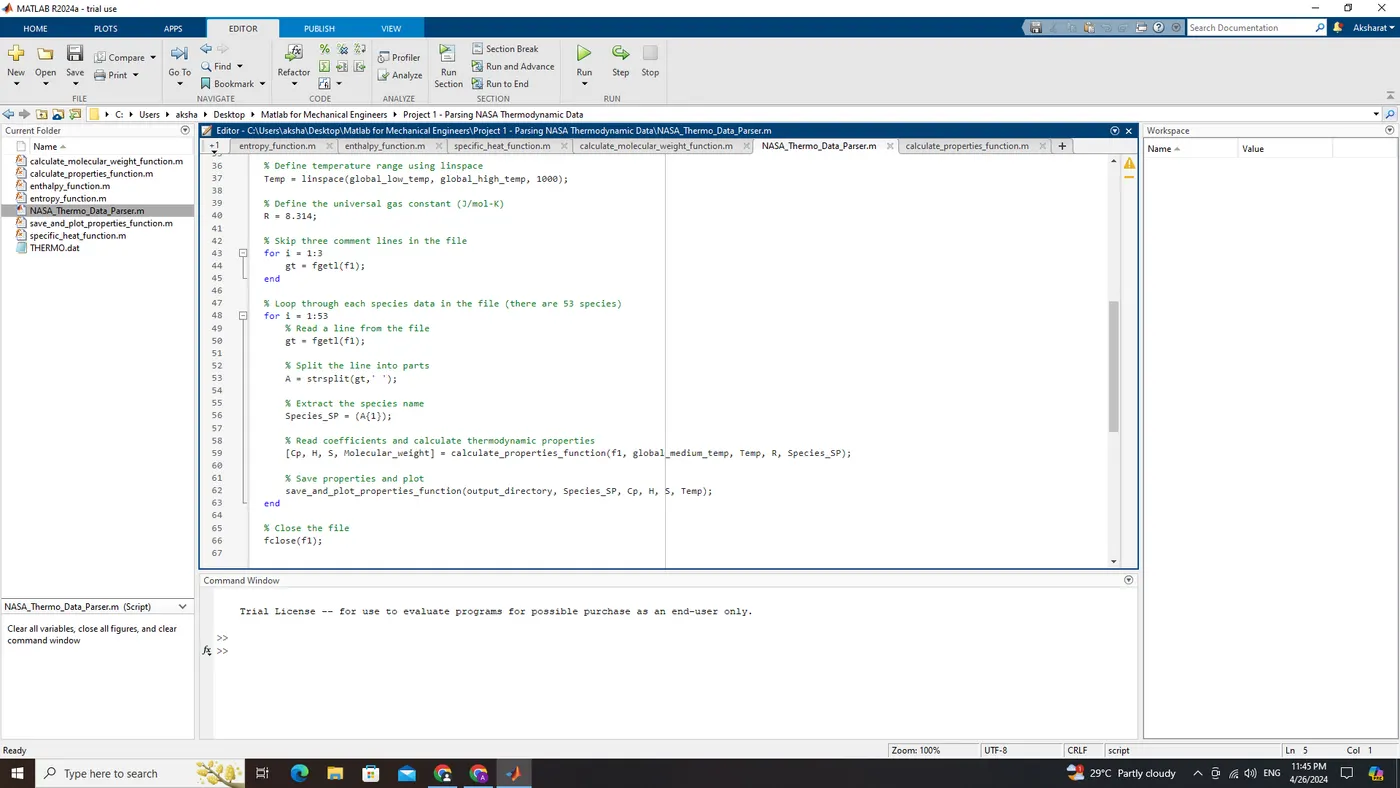
% Loop through each species data in the file (there are 53 species)
for i = 1:53
    % Read a line from the file
    gt = fgetl(f1);
    
    % Split the line into parts
    A = strsplit(gt,' ');
    
    % Extract the species name
    Species_SP = (A{1});

    % Read coefficients and calculate thermodynamic properties
    [Cp, H, S, Molecular_weight] = calculate_properties_function(f1, global_medium_temp, Temp, R, Species_SP);

    % Save properties and plot
    save_and_plot_properties_function(output_directory, Species_SP, Cp, H, S, Temp);
end

% Close the file
fclose(f1);

Explanation:

Initialization and File Handling

clear all
close all
clc

output_directory = 'C:\Users\aksha\Desktop\Matlab for Mechanical Engineers\Project 1 - Parsing NASA Thermodynamic Data';
mkdir(output_directory);

f1 = fopen('THERMO.dat','r');

gt = fgetl(f1);

Here, the code begins by clearing all variables, closing all figures, and clearing the command window. Then, it defines a directory output_directory where output files will be stored. The code opens a file named THERMO.dat in read mode ('r') and reads the first line of the file into the variable gt.

Parsing Temperature Range Information

global_temp = fgetl(f1);

t = strsplit(global_temp);

global_low_temp = str2double(t{2});
global_medium_temp = str2double(t{3});
global_high_temp = str2double(t{4});

This section reads the temperature range information from the file's header, splits it into parts, and converts the temperature range strings into numerical values (global_low_temp, global_medium_temp, and global_high_temp).

Temperature Range Definition

Temp = linspace(global_low_temp, global_high_temp, 1000);

Using the obtained temperature range, this part generates a linearly spaced vector Temp with 1000 points between global_low_temp and global_high_temp.

Constants Definition

R = 8.314;

The code defines the universal gas constant R with a value of 8.314 J/(mol·K).

Skipping Comment Lines

for i = 1:3
    gt = fgetl(f1);
end

This loop iterates three times to skip over three comment lines in the file.

Processing Species Data

for i = 1:53
    gt = fgetl(f1);
    A = strsplit(gt,' ');
    Species_SP = (A{1});
    [Cp, H, S, Molecular_weight] = calculate_properties_function(f1, global_medium_temp, Temp, R, Species_SP);
    save_and_plot_properties_function(output_directory, Species_SP, Cp, H, S, Temp);
end

This loop iterates over each species data in the file. It reads a line, splits it into parts, extracts the species name, calls a function calculate_properties_function to compute thermodynamic properties (Cp, H, S, Molecular_weight), and then calls another function save_and_plot_properties_function to save properties and plot them.

Closing File

fclose(f1);

Finally, the code closes the file f1 after processing all the species data.

This code is parsing NASA Thermodynamic data, calculating thermodynamic properties for each species, and saving/plottin them in the specified output directory.

////

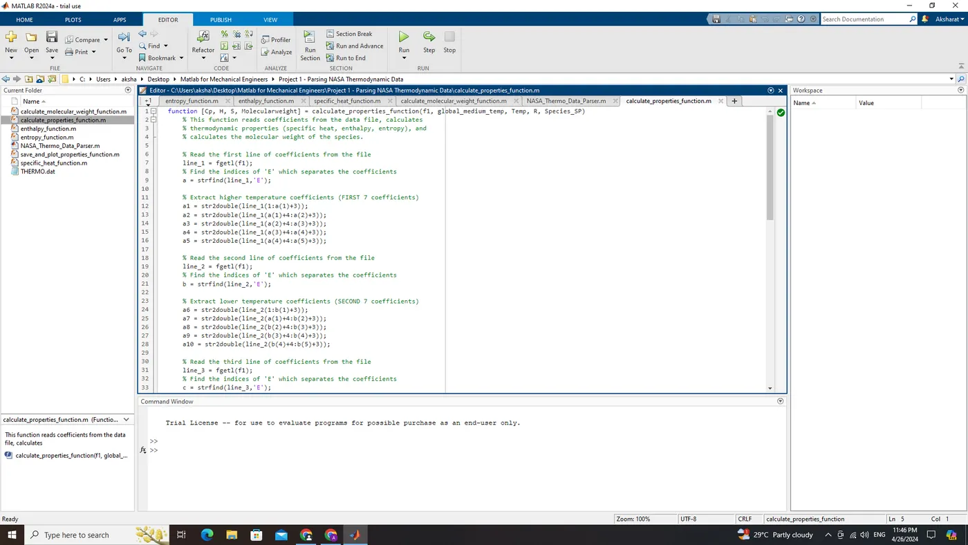
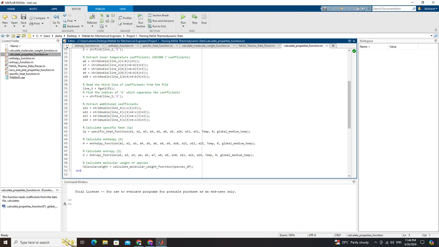
calculate_properties_function

function [Cp, H, S, Molecularweight] = calculate_properties_function(f1, global_medium_temp, Temp, R, Species_SP)
    % This function reads coefficients from the data file, calculates
    % thermodynamic properties (specific heat, enthalpy, entropy), and
    % calculates the molecular weight of the species.

    % Read the first line of coefficients from the file
    line_1 = fgetl(f1);        
    % Find the indices of 'E' which separates the coefficients
    a = strfind(line_1,'E');

    % Extract higher temperature coefficients (FIRST 7 coefficients)
    a1 = str2double(line_1(1:a(1)+3));
    a2 = str2double(line_1(a(1)+4:a(2)+3));
    a3 = str2double(line_1(a(2)+4:a(3)+3));
    a4 = str2double(line_1(a(3)+4:a(4)+3));
    a5 = str2double(line_1(a(4)+4:a(5)+3));

    % Read the second line of coefficients from the file
    line_2 = fgetl(f1);
    % Find the indices of 'E' which separates the coefficients
    b = strfind(line_2,'E');

    % Extract lower temperature coefficients (SECOND 7 coefficients)
    a6 = str2double(line_2(1:b(1)+3));
    a7 = str2double(line_2(a(1)+4:b(2)+3));
    a8 = str2double(line_2(b(2)+4:b(3)+3));         
    a9 = str2double(line_2(b(3)+4:b(4)+3));
    a10 = str2double(line_2(b(4)+4:b(5)+3));

    % Read the third line of coefficients from the file
    line_3 = fgetl(f1);
    % Find the indices of 'E' which separates the coefficients
    c = strfind(line_3,'E');

    % Extract additional coefficients
    a11 = str2double(line_3(1:c(1)+3));
    a12 = str2double(line_3(c(1)+4:c(2)+3));
    a13 = str2double(line_3(c(2)+4:c(3)+3));
    a14 = str2double(line_3(c(3)+4:c(4)+3));

    % Calculate specific heat (Cp)
    Cp = specific_heat_function(a1, a2, a3, a4, a5, a8, a9, a10, a11, a12, Temp, R, global_medium_temp);

    % Calculate enthalpy (H)
    H = enthalpy_function(a1, a2, a3, a4, a5, a6, a8, a9, a10, a11, a12, a13, Temp, R, global_medium_temp);

    % Calculate entropy (S)
    S = entropy_function(a1, a2, a3, a4, a5, a7, a8, a9, a10, a11, a12, a14, Temp, R, global_medium_temp);

    % Calculate molecular weight of species
    Molecularweight = calculate_molecular_weight_function(Species_SP);
end

Explanation:

Function Definition

function [Cp, H, S, Molecularweight] = calculate_properties_function(f1, global_medium_temp, Temp, R, Species_SP)

This defines a MATLAB function named calculate_properties_function with input arguments f1, global_medium_temp, Temp, R, and Species_SP, and output arguments Cp, H, S, and Molecularweight.

Function Description

% This function reads coefficients from the data file, calculates
% thermodynamic properties (specific heat, enthalpy, entropy), and
% calculates the molecular weight of the species.

This comment describes the purpose of the function, which is to read coefficients from a data file, calculate thermodynamic properties (specific heat, enthalpy, entropy), and calculate the molecular weight of the species.

Reading Coefficients from Data File

    % Read the first line of coefficients from the file
    line_1 = fgetl(f1);        
    % Find the indices of 'E' which separates the coefficients
    a = strfind(line_1,'E');

    % Extract higher temperature coefficients (FIRST 7 coefficients)
    a1 = str2double(line_1(1:a(1)+3));
    a2 = str2double(line_1(a(1)+4:a(2)+3));
    a3 = str2double(line_1(a(2)+4:a(3)+3));
    a4 = str2double(line_1(a(3)+4:a(4)+3));
    a5 = str2double(line_1(a(4)+4:a(5)+3));

    % Read the second line of coefficients from the file
    line_2 = fgetl(f1);
    % Find the indices of 'E' which separates the coefficients
    b = strfind(line_2,'E');

    % Extract lower temperature coefficients (SECOND 7 coefficients)
    a6 = str2double(line_2(1:b(1)+3));
    a7 = str2double(line_2(a(1)+4:b(2)+3));
    a8 = str2double(line_2(b(2)+4:b(3)+3));         
    a9 = str2double(line_2(b(3)+4:b(4)+3));
    a10 = str2double(line_2(b(4)+4:b(5)+3));

    % Read the third line of coefficients from the file
    line_3 = fgetl(f1);
    % Find the indices of 'E' which separates the coefficients
    c = strfind(line_3,'E');

    % Extract additional coefficients
    a11 = str2double(line_3(1:c(1)+3));
    a12 = str2double(line_3(c(1)+4:c(2)+3));
    a13 = str2double(line_3(c(2)+4:c(3)+3));
    a14 = str2double(line_3(c(3)+4:c(4)+3));

This section reads the coefficients from the data file (f1) and extracts them from each line. It uses the positions of 'E' in each line to split the coefficients correctly.

Calculating Specific Heat (Cp)

    Cp = specific_heat_function(a1, a2, a3, a4, a5, a8, a9, a10, a11, a12, Temp, R, global_medium_temp);

This line calculates the specific heat (Cp) using the coefficients extracted from the data file and the specific_heat_function.

Calculating Enthalpy (H)

    H = enthalpy_function(a1, a2, a3, a4, a5, a6, a8, a9, a10, a11, a12, a13, Temp, R, global_medium_temp);

This line calculates the enthalpy (H) using the coefficients extracted from the data file and the enthalpy_function.

Calculating Entropy (S)

    S = entropy_function(a1, a2, a3, a4, a5, a7, a8, a9, a10, a11, a12, a14, Temp, R, global_medium_temp);

This line calculates the entropy (S) using the coefficients extracted from the data file and the entropy_function.

Calculating Molecular Weight

    Molecularweight = calculate_molecular_weight_function(Species_SP);

This line calculates the molecular weight of the species using the calculate_molecular_weight_function.

Function Output

end

This marks the end of the function definition.

Overall, this function reads coefficients from a data file, calculates thermodynamic properties (specific heat, enthalpy, entropy), and calculates the molecular weight of the species using the provided functions

////

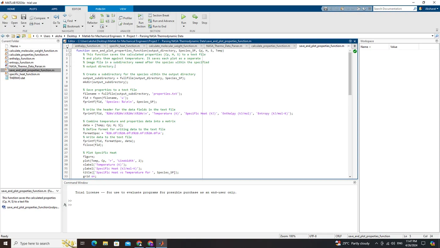
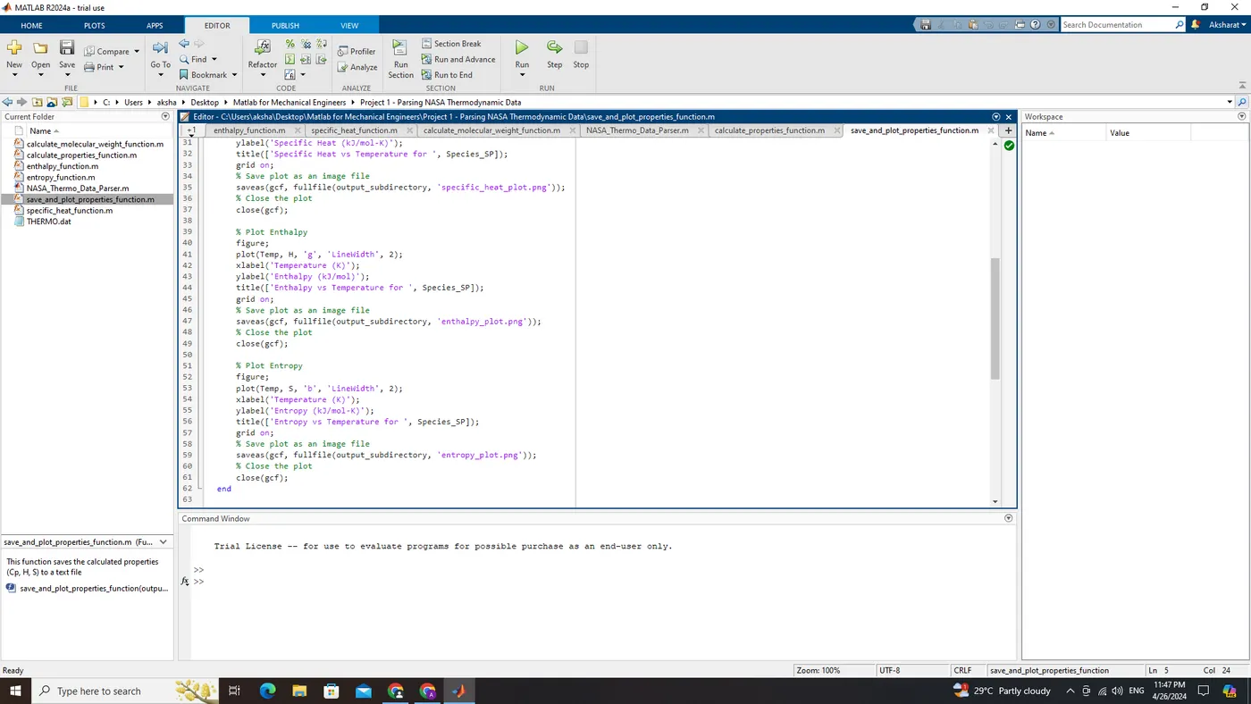
save_and_plot_properties_function

function save_and_plot_properties_function(output_directory, Species_SP, Cp, H, S, Temp)
    % This function saves the calculated properties (Cp, H, S) to a text file 
    % and plots them against temperature. It saves each plot as a separate 
    % image file in a subdirectory named after the species within the specified 
    % output directory.

    % Create a subdirectory for the species within the output directory
    output_subdirectory = fullfile(output_directory, Species_SP);
    mkdir(output_subdirectory);

    % Save properties to a text file
    filename = fullfile(output_subdirectory, 'properties.txt');
    fid = fopen(filename, 'w');
    fprintf(fid, 'Species: %s\n\n', Species_SP);

    % Write the header for the data fields in the text file
    fprintf(fid, '%20s\t%20s\t%20s\t%20s\n', 'Temperature (K)', 'Specific Heat (kJ)', 'Enthalpy (kJ/mol)', 'Entropy (kJ/mol-K)');

    % Combine temperature and properties data into a matrix
    data = [Temp; Cp; H; S];
    % Define format for writing data to the text file
    formatSpec = '%20.6f\t%20.6f\t%20.6f\t%20.6f\n';
    % Write data to the text file
    fprintf(fid, formatSpec, data);
    fclose(fid);

    % Plot Specific Heat
    figure;
    plot(Temp, Cp, 'r', 'LineWidth', 2);
    xlabel('Temperature (K)');
    ylabel('Specific Heat (kJ/mol-K)');
    title(['Specific Heat vs Temperature for ', Species_SP]);
    grid on;
    % Save plot as an image file
    saveas(gcf, fullfile(output_subdirectory, 'specific_heat_plot.png'));
    % Close the plot
    close(gcf);

    % Plot Enthalpy
    figure;
    plot(Temp, H, 'g', 'LineWidth', 2);
    xlabel('Temperature (K)');
    ylabel('Enthalpy (kJ/mol)');
    title(['Enthalpy vs Temperature for ', Species_SP]);
    grid on;
    % Save plot as an image file
    saveas(gcf, fullfile(output_subdirectory, 'enthalpy_plot.png'));
    % Close the plot
    close(gcf);

    % Plot Entropy
    figure;
    plot(Temp, S, 'b', 'LineWidth', 2);
    xlabel('Temperature (K)');
    ylabel('Entropy (kJ/mol-K)');
    title(['Entropy vs Temperature for ', Species_SP]);
    grid on;
    % Save plot as an image file
    saveas(gcf, fullfile(output_subdirectory, 'entropy_plot.png'));
    % Close the plot
    close(gcf);
end

Explanation:

Function Definition

function save_and_plot_properties_function(output_directory, Species_SP, Cp, H, S, Temp)

This function named save_and_plot_properties_function takes six input arguments: output_directory, Species_SP, Cp, H, S, and Temp.

Function Description

    % This function saves the calculated properties (Cp, H, S) to a text file 
    % and plots them against temperature. It saves each plot as a separate 
    % image file in a subdirectory named after the species within the specified 
    % output directory.

This comment describes the purpose of the function, which is to save the calculated thermodynamic properties (specific heat Cp, enthalpy H, and entropy S) to a text file and plot them against temperature. It also specifies that each plot will be saved as a separate image file in a subdirectory named after the species within the specified output directory.

Creating Subdirectory

    output_subdirectory = fullfile(output_directory, Species_SP);
    mkdir(output_subdirectory);

This section creates a subdirectory named after the species (Species_SP) within the specified output directory (output_directory) using mkdir.

Saving Properties to Text File

    filename = fullfile(output_subdirectory, 'properties.txt');
    fid = fopen(filename, 'w');
    fprintf(fid, 'Species: %s\n\n', Species_SP);

    fprintf(fid, '%20s\t%20s\t%20s\t%20s\n', 'Temperature (K)', 'Specific Heat (kJ)', 'Enthalpy (kJ/mol)', 'Entropy (kJ/mol-K)');

    data = [Temp; Cp; H; S];
    formatSpec = '%20.6f\t%20.6f\t%20.6f\t%20.6f\n';
    fprintf(fid, formatSpec, data);
    fclose(fid);

This part creates and opens a text file named properties.txt within the species subdirectory. It writes the species name, a header for the data fields, and then writes the temperature and properties data (specific heat, enthalpy, and entropy) to the text file.

Plotting and Saving Specific Heat Plot

    figure;
    plot(Temp, Cp, 'r', 'LineWidth', 2);
    xlabel('Temperature (K)');
    ylabel('Specific Heat (kJ/mol-K)');
    title(['Specific Heat vs Temperature for ', Species_SP]);
    grid on;
    saveas(gcf, fullfile(output_subdirectory, 'specific_heat_plot.png'));
    close(gcf);

This section plots the specific heat (Cp) against temperature and customizes the plot appearance. It saves the plot as an image file named specific_heat_plot.png within the species subdirectory.

Plotting and Saving Enthalpy Plot

    figure;
    plot(Temp, H, 'g', 'LineWidth', 2);
    xlabel('Temperature (K)');
    ylabel('Enthalpy (kJ/mol)');
    title(['Enthalpy vs Temperature for ', Species_SP]);
    grid on;
    saveas(gcf, fullfile(output_subdirectory, 'enthalpy_plot.png'));
    close(gcf);

This part plots the enthalpy (H) against temperature, customizes the plot appearance, saves the plot as an image file named enthalpy_plot.png within the species subdirectory, and then closes the plot window.

Plotting and Saving Entropy Plot

    figure;
    plot(Temp, S, 'b', 'LineWidth', 2);
    xlabel('Temperature (K)');
    ylabel('Entropy (kJ/mol-K)');
    title(['Entropy vs Temperature for ', Species_SP]);
    grid on;
    saveas(gcf, fullfile(output_subdirectory, 'entropy_plot.png'));
    close(gcf);

This section plots the entropy (S) against temperature, customizes the plot appearance, saves the plot as an image file named entropy_plot.png within the species subdirectory, and then closes the plot window.

Function Output

end

This marks the end of the function definition.

Overall, this function creates a subdirectory for the species, saves the calculated thermodynamic properties to a text file within that subdirectory, and plots each property against temperature, saving each plot as a separate image file within the species subdirectory.

////

Let's break down the logic behind each of the provided functions:

calculate_molecular_weight_function:

Initialization: Initialize variables for atomic names and corresponding atomic weights.
Iteration: Iterate over each character in the chemical formula (Species_SP).
Matching: Match each character with standard atomic names to find the corresponding atomic weight.
Accumulation: Accumulate the atomic weights to calculate the total molecular weight.
Output: Display the calculated molecular weight.

entropy_function, enthalpy_function, specific_heat_function:

Temperature Range Check: Check if the temperature is within the low or high temperature range.
Coefficient Extraction: Extract the coefficients for the appropriate temperature range from the provided data.
Calculation: Use the extracted coefficients to calculate the respective thermodynamic property (entropy, enthalpy, specific heat) based on the temperature.
Output: Return the calculated property.

calculate_properties_function:

Coefficient Extraction: Read coefficients for specific species from the provided file.
Property Calculation: Calculate thermodynamic properties (specific heat, enthalpy, entropy) using the extracted coefficients and the respective functions.
Molecular Weight Calculation: Calculate the molecular weight of the species using the provided function.
Output: Return the calculated properties and molecular weight.

save_and_plot_properties_function:

Subdirectory Creation: Create a subdirectory for the species within the output directory.
Property Saving: Save the calculated properties (specific heat, enthalpy, entropy) along with temperature to a text file within the subdirectory.
Plotting: Plot each property against temperature, customize the appearance, save the plots as image files within the subdirectory.

Overall Logic:

Data Input: Read input data (coefficients, species information).
Property Calculation: Use the provided coefficients and functions to calculate thermodynamic properties and molecular weight.
Data Output: Save calculated properties to a text file and plot them against temperature, saving each plot as an image file.
Organization: Organize data and results by creating subdirectories for each species within the output directory.

By following this logic, the provided functions efficiently handle the input data, perform calculations, and organize the output for further analysis and visualization.

Output:

entropy_function

enthalpy_function

specific_heat_function

calculate_molecular_weight_function

NASA_Thermo_Data_Parser

calculate_properties_function

save_and_plot_properties_function

NASA Thermodynamic Data File

Output Results:

////

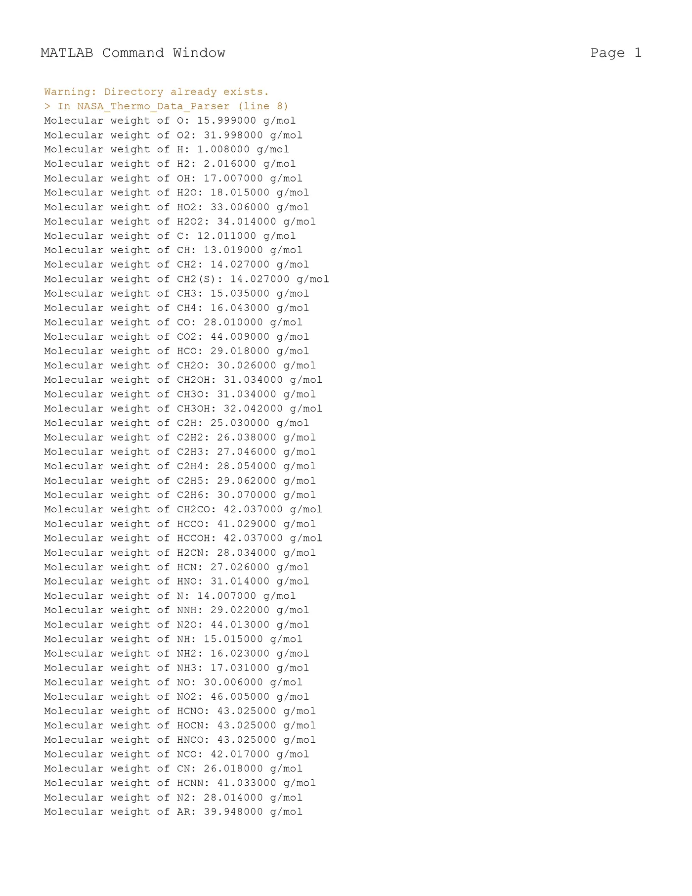
Plots for O2

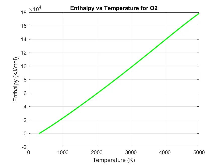
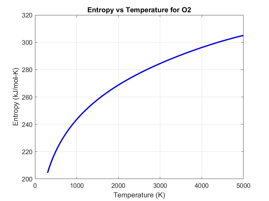
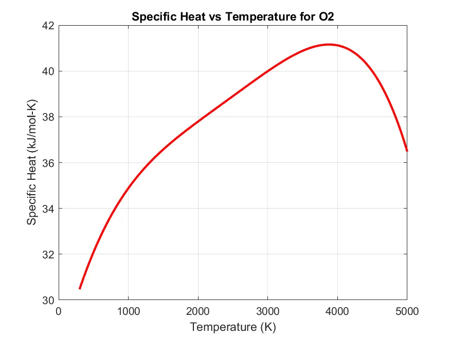
Plots for N2

Plots for CO2

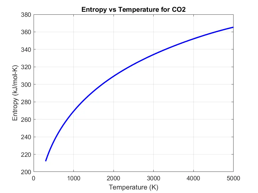
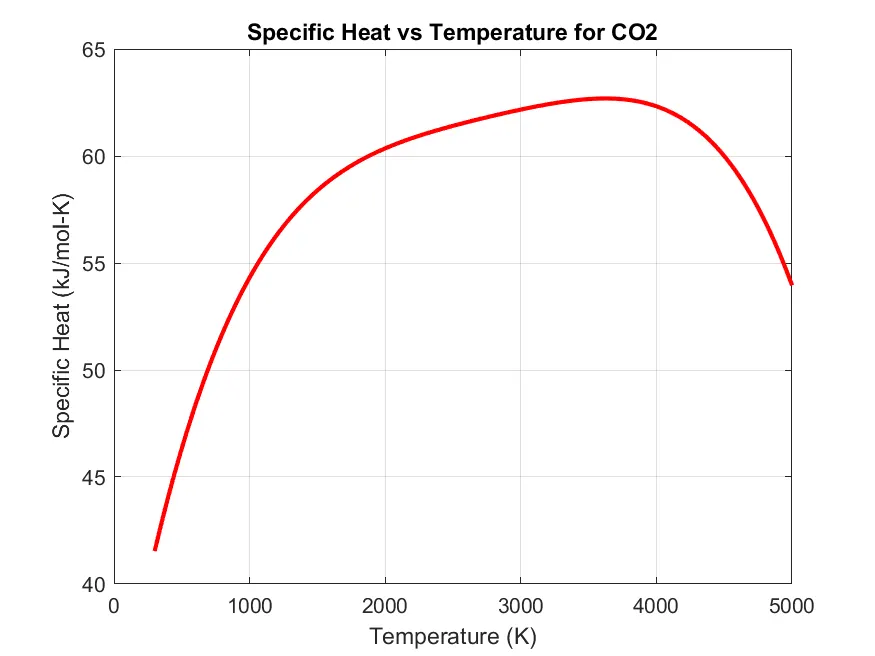
Extras:

I have also done one extra work by grouping all the calculated thermodynamic properties values of Specific Heat (kJ), Enthalpy (kJ/mol), Entropy (kJ/mol-K) of a given chemical species over a range of temperature into a file called "properties.txt".

Conclusion:

In this project, we developed a MATLAB program for parsing NASA thermodynamic data and analyzing thermodynamic properties of various species. The project involved several key components:

Data Parsing and Extraction: We parsed NASA thermodynamic data files to extract coefficients representing the thermodynamic properties of different chemical species over specified temperature ranges.
Thermodynamic Property Calculation: Utilizing the extracted coefficients, we implemented functions to calculate specific thermodynamic properties such as specific heat, enthalpy, and entropy for each species over a range of temperatures.
Molecular Weight Calculation: Additionally, we incorporated a function to calculate the molecular weight of each species based on its chemical formula.
Data Visualization and Analysis: To visualize the thermodynamic properties, we generated plots of specific heat, enthalpy, and entropy against temperature for each species. These plots provide insights into the behavior of each species as a function of temperature.
Data Organization and Storage: Finally, we organized the calculated properties and plots by creating subdirectories for each species within the output directory. This ensures that the results are easily accessible and organized for further analysis.

Overall, this project provides a comprehensive framework for parsing NASA thermodynamic data, calculating thermodynamic properties, and visualizing the results. It can serve as a valuable tool for researchers and engineers working in fields such as aerospace engineering, chemical engineering, and materials science, where understanding thermodynamic properties of species is essential for design and analysis.

Project 1 - Parsing NASA thermodynamic data

Ship work like this
in your own course.

Talk to a career counsellor

Ship work like thisin your own course.

Talk to a career counsellor

Ship work like this
in your own course.