Project 1 - Parsing NASA thermodynamic data
THE CODE:
The logic of the code is explained linewise in the matlab code itslef
clear all
clc
close all

f1=fopen('THERMO.dat','r'); %opens THERMO.dat file as a readable file
r=8.3145; % Universal gas constant
%% Obtaining Line-wise Data
for i = 1 : 218 %since there are 218 rows in the THERMo.dat file
A{i,1}=fgetl(f1); %to go through the lines and store each line in a cell named A, each row is a line from THERMO.dat file stored as string
    if i == 2 % since global maximum and minimum temperatures were in 2nd row
        Z=strsplit(A{2},' '); %the string is split where the corresponding string character is found
        %global temperature range
        Global_minimum=str2num(Z{2}); %converts string character into number
        Global_medium=str2num(Z{3});
        Global_maximum=str2num(Z{4});
    end

end


%% Parsing the data
c=0; %c is the counter, since we have the data in a repetetive order in the THERMO.dat file, this will be used in the loop
i=7; %the coefficient data starts from line 7 until line 217, with 3 lines of coeffiecents followed by a line of species header and so it repeats.
k=1; % used to store the data in a more readable tabular format, value of k corresponds to the row index of the array in which the coefficients are stored
while  7 <= i && i <= 217
    D=A{i}; %temporarily stores the line of data from THERMO.dat, so that data could be parsed from it
    c=c+1; %each time we go through loop c value goes from 1 to 3, where c corresponds to the line of coefficient data for eaach species
    %for each species, the coefficients are stored in three lines and c corresponds to each line
    if c == 1
         % x temporarily stores first 7 coefficients of the particular species, this coreesponds to the high temperature coefficients
         % first 5 coefficeints are in line 1 (c=1) for each species
    x{1}=D(1:15);
    x{2}=D(16:30);
    x{3}=D(31:45);
    x{4}=D(46:60);
    x{5}=D(61:75);
    end
    if c == 2
        % 6 and 7th coefficeints are in line 2 (c=2) for each species
    x{6}=D(1:15);
    x{7}=D(16:30);
        % y temporarily stores the next 7 coefficients of the particular species, this coreesponds to the low temperature coefficients
        % coefficients 8 to 10 are in line 2 (c=2) for each species
    y{1}=D(31:45);
    y{2}=D(46:60);
    y{3}=D(61:75);
    end
    if c == 3
        % coefficeints 11 to 14 are in line 3 (c=3) for each species
    y{4}=D(1:15);
    y{5}=D(16:30);
    y{6}=D(31:45);
    y{7}=D(46:60);
     i=i+1; %after the third line of each species, the next line is the header of next species, inorder to skip it, i is increased by 1 before hand
     c=0; % resets value of c to 0 so that when it goes to next species c starts from 1
     for j = 1 : 7
         X(k,j)=str2num(x{j}); %High Temperature Coefficients stored as an array in X
         Y(k,j)=str2num(y{j}); %Low Temperature Coefficients stored as an array in Y
     end
     k=k+1; % to store the coefficients of next species in the next row of array X and Y
    end

    i=i+1; % to go to the next line
end

%% Matching Data to corresponding species
High_Coeff=cell(54,8); % creating cell so that we can have a tabular format, to visualize corresponding data for each species
Low_Coeff=cell(54,8);
for i= 1: length(X)
    for j = 2 :width(High_Coeff)
    High_Coeff{i+1,j}=X(i,j-1); % assigning values from array X to Cell named High_Coeff
    Low_Coeff{i+1,j}=Y(i,j-1); % assigning values from array Y to Cell named Low_Coeff
    end
end

%to get species name and molecular mass
for i = 6 : 4 : 214
  %To match corresponding species
    D=A{i}; % temporary variable in which character is stored to analyze and get data from
    High_Coeff{1+((i-2)/4),1}=D(1:6); % the name of species is stored is first 6 lines of D
    Low_Coeff{1+((i-2)/4),1}=D(1:6); % the name of species is stored is first 6 lines of D
 %to find molecular mass
 %first six character spaces are used to define the species in the THERMO.dat file
 %the only elements in the species are the elements listed below
 %we create an array s, where each row corresponds to each species
 %the size of columns corresponds to the length of characters, i.e. 6
 %each character is observed and according to it the mass of it is stored in the array
 %the subscripts are multiplied to the previous element and the column corresponding to the subscript is stored as zero
 % Brackets and spaces are also stored as 0, finally the sum of each species is calculated by summing up the columns of each rows
    for j = 1 : 6
    if D(j)=='H'
    s(1+((i-2)/4),j)=1; %mass of H
elseif D(j)=='O'
    s(1+((i-2)/4),j)=16; %mass of O
elseif D(j)=='S'
    s(1+((i-2)/4),j)=32.065; %mass of S
elseif D(j)=='C'
    s(1+((i-2)/4),j)=12.011; %mass of C
elseif D(j)=='N'
    s(1+((i-2)/4),j)=14; %mass of N
elseif D(j)=='A'
    s(1+((i-2)/4),j)=39.948; %mass of Ar
elseif D(j)=='R'
    s(1+((i-2)/4),j)=0; %mass of Argon stored in A
elseif D(j)==' ' || D(j)=='(' || D(j)==')'
    s(1+((i-2)/4),j)=0; %values assigned for space and brackets
else
    s(1+((i-2)/4),j)=str2num(D(j)); %value of subscripts
    s(1+((i-2)/4),j-1)=s(1+((i-2)/4),j-1)*s(1+((i-2)/4),j); %multiplying subscripts with corresponding elements
    s(1+((i-2)/4),j)=0; % storing value to the subscript space as 0
    end
    end
end

%To make it into a table format, giving headings
High_Coeff{1,1}='Species';
Low_Coeff{1,1}='Species';
High_Coeff{1,2}='a1';
Low_Coeff{1,2}='a1';
High_Coeff{1,3}='a2';
Low_Coeff{1,3}='a2';
High_Coeff{1,4}='a3';
Low_Coeff{1,4}='a3';
High_Coeff{1,5}='a4';
Low_Coeff{1,5}='a4';
High_Coeff{1,6}='a5';
Low_Coeff{1,6}='a5';
High_Coeff{1,7}='a6';
Low_Coeff{1,7}='a6';
High_Coeff{1,8}='a7';
Low_Coeff{1,8}='a7';

%obtaining local low and high temperature as string
%low and high temperatures are in the 49-55 position and 58 to 66 position
%of the THERMO.dat file in lines 6, 10, 14 .... till 214
for i = 6 : 4 : 214
    D=A{i}; %temporary variable from which data is obtained
    Low_temp{1+((i-2)/4),1}=D(49:55); %low temperature as string
    High_temp{1+((i-2)/4),1}=D(58:66); %high temperature as string
    Transition_temp{1+((i-2)/4),1}=D(68:76); %transition temperature from low to high coefficients
end

Low_temp{1}='Low Temp';
High_temp{1}='High Temp';
Transition_temp{1}='Transition Temp';
%conversion into number
for i = 2 : 54
    Low_temp{i}=str2num(Low_temp{i}); % conversion into number from string to get the Low local temperature
    High_temp{i}=str2num(High_temp{i}); % conversion into number from string to get the high local temperature
    Transition_temp{i}=str2num(Transition_temp{i}); % conversion into number from string to get the transition local temperature
end
Temp=cell(54,3); % To store all the local temperature data in one cell named Temp, each rows of data in Temp corresponds to each row of species in the cells named C, High_Coeff, and Low_Coeff
Temp(:,1)=Low_temp(:,1); % first column for low local temperatures
Temp(:,2)=Transition_temp(:,1); % second column for transition local temperatures
Temp(:,3)=High_temp(:,1); % third column for high local temperatures
%% Calculations

%if C cell is copened we can see table format arrangement of data

%Let C be the  Calculation cell

C(:,1)=High_Coeff(:,1); % Species name, so that the Cell is easy to read


%Givivng headings to represent the cell C in a tabular format
C{1,2}='Cp';
C{1,3}='H';
C{1,4}='S';
C{1,5}='Molecular Weight';

%To calculate molecular weight
for i = 2 : 54
    % The fifth colum of C corresponds to Molecular weight of the species
    C{i,5}=s(i,1); % where s(i,1) is the molecular weight of the first element in the speices
    for j = 2 : width(s)
    C{i,5}=C{i,5}+s(i,j); % addition of molecular weight of subsequent elements to get total molecular weight of the species
    end
end

%Calculating C

for i = 2 : 54
    c=1;  % c is the row number corresponding to the temperature at which the calculations are carried out
           %  (max number of c for each element is the maximum is (High_temp - Low_temp)+1 )
           % this is done so, that we can plot the Cp, H, and S vs Temperature graphs
    for j = Temp{i,1} : 1 : Temp{i,3}
        if j > Temp{i,2} % the temperature above which we start using High Temperature Coefficients
            %C{i,2} calculates specific heat for high temperatures
C{i,2}(c,1) = (High_Coeff{i,2} + (High_Coeff{i,3}*j) + (High_Coeff{i,4}*j^2) + (High_Coeff{i,5}*j^3) + (High_Coeff{i,6}*j^4))*(r/(C{i,5}/1000));
            %C{i,3} calculates Enthalpy for high temperatures
C{i,3}(c,1) = (High_Coeff{i,2} + (High_Coeff{i,3}*j/2) + (High_Coeff{i,4}*(j^2)/3) + (High_Coeff{i,5}*(j^3)/4) + (High_Coeff{i,6}*(j^4)/5) + (High_Coeff{i,7}/j))*(r/(C{i,5}/1000))*j;
            %C{i,4} calculates Entropy for high temperatures
C{i,4}(c,1) = ((High_Coeff{i,2}*log(j)) + (High_Coeff{i,3}*j) + (High_Coeff{i,4}*(j^2)/2) + (High_Coeff{i,5}*(j^3)/3) + (High_Coeff{i,6}*(j^4)/4) + High_Coeff{i,8})*(r/(C{i,5}/1000));
        else
            %C{i,2} calculates specific heat for high temperatures
C{i,2}(c,1) = (Low_Coeff{i,2} + (Low_Coeff{i,3}*j) + (Low_Coeff{i,4}*j^2) + (Low_Coeff{i,5}*j^3) + (Low_Coeff{i,6}*j^4))*(r/(C{i,5}/1000));
            %C{i,3} calculates Enthalpy for high temperatures
C{i,3}(c,1) = (Low_Coeff{i,2} + (Low_Coeff{i,3}*j/2) + (Low_Coeff{i,4}*(j^2)/3) + (Low_Coeff{i,5}*(j^3)/4) + (Low_Coeff{i,6}*(j^4)/5) + (Low_Coeff{i,7}/j))*(r/(C{i,5}/1000))*j;
            %C{i,4} calculates Entropy for high temperatures
C{i,4}(c,1) = ((Low_Coeff{i,2}*log(j)) + (Low_Coeff{i,3}*j) + (Low_Coeff{i,4}*(j^2)/2) + (Low_Coeff{i,5}*(j^3)/3) + (Low_Coeff{i,6}*(j^4)/4) + Low_Coeff{i,8})*(r/(C{i,5}/1000));
        end
c=c+1;
    end % the loop calculates for each and every temperature starting from Low temperature all the way upto the highest temperature
end %this for loop ensures calculations are done to each and every species

%% Printing answers and plotting data

for i = 2 : 54

    %The automated plotting code
    T=Temp{i,1} : 1 :Temp{i,3}; % the array of temperature range for each species, data is overwrited on each iteration of loop to the required temperature ranges corresponding the the species

    %figure windows for specific heat, enthalpy, and entropy are called
    %so that they can be closed after plotting. If left open it would cause the Matlab program to lag as 159 windows of figures will be opened by Matlab

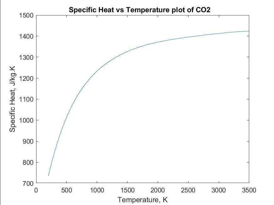
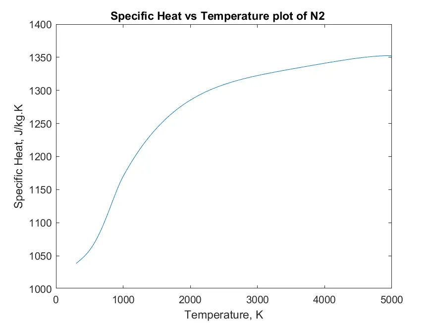
    cp=figure('Name',['Specific Heat vs Temperature plot of ', C{i,1}]); % figure window for Enthalpy
    z=C{i,2}; % Specific heat data temporarily stored in z
    plot(T,z); % command to plot the required graph Specific Heat vs Temperature
    title(['Specific Heat vs Temperature plot of ', C{i,1}])
    xlabel('Temperature, K')
    ylabel('Specific Heat, J/kg.K')
    saveas(cp,['Specific Heat vs Temperature plot of ', C{i,1},'.png']) % automatically saves the figure as the specified file (here .png image file)
    close(cp) % closes the figure of Specific heat vs Temperature

    %the syntax for enthalpy and entropy are the same as specific heat

    H=figure('Name',['Enthalpy vs Temperature plot of ', C{i,1}]);
    z=C{i,3};
    plot(T,z);
    title(['Enthalpy vs Temperature plot of ', C{i,1}])
    xlabel('Temperature, K')
    ylabel('Enthalpy, J/kg')
    saveas(H,['Enthalpy vs Temperature plot of ', C{i,1},'.png'])
    close(H)

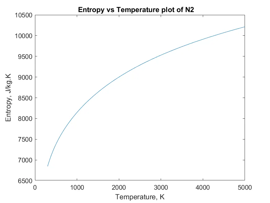
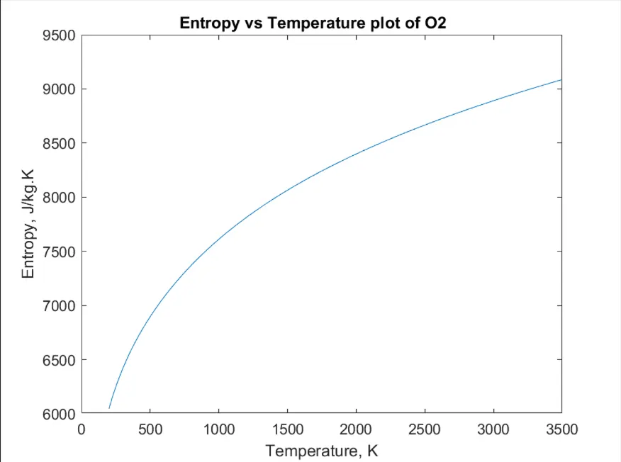
    S=figure('Name',['Entropy vs Temperature plot of ', C{i,1}]);
    z=C{i,4};
    plot(T,z);
    title(['Entropy vs Temperature plot of ', C{i,1}])
    xlabel('Temperature, K')
    ylabel('Entropy, J/kg.K')
    saveas(S,['Entropy vs Temperature plot of ', C{i,1},'.png'])
    close(S)

    %The printing code

    %since the molecular names in first column of cell C is saved as strings and since the space characters
    % in the string was not excluded while storing the string value in cell C, we split the string
    % where we find the space character by the following command
    zoo{i,1}=strsplit(C{i,1},' '); % this is saved into a cell named zoo which just contains the species name in its rows without ' ' character
    fprintf(['The Molecular weight of species ',zoo{i,1}{1,1},' is %0.4f\n'],C{i,5}) % the molecular weight stored in fifth column of C is printed

end
SCREENSHOTS:
Molecular weight of each speices displayed in command window:
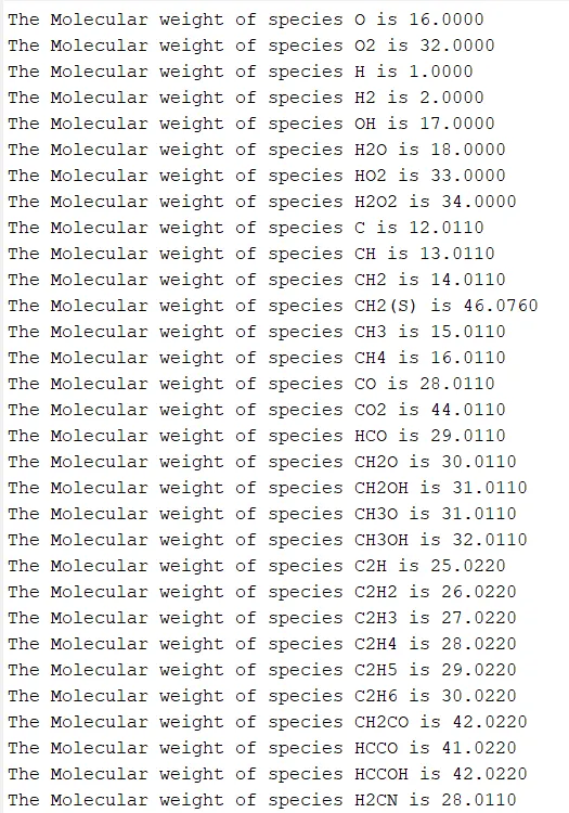
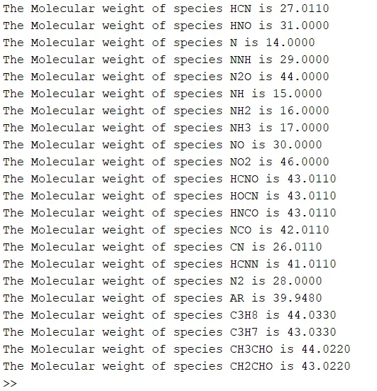
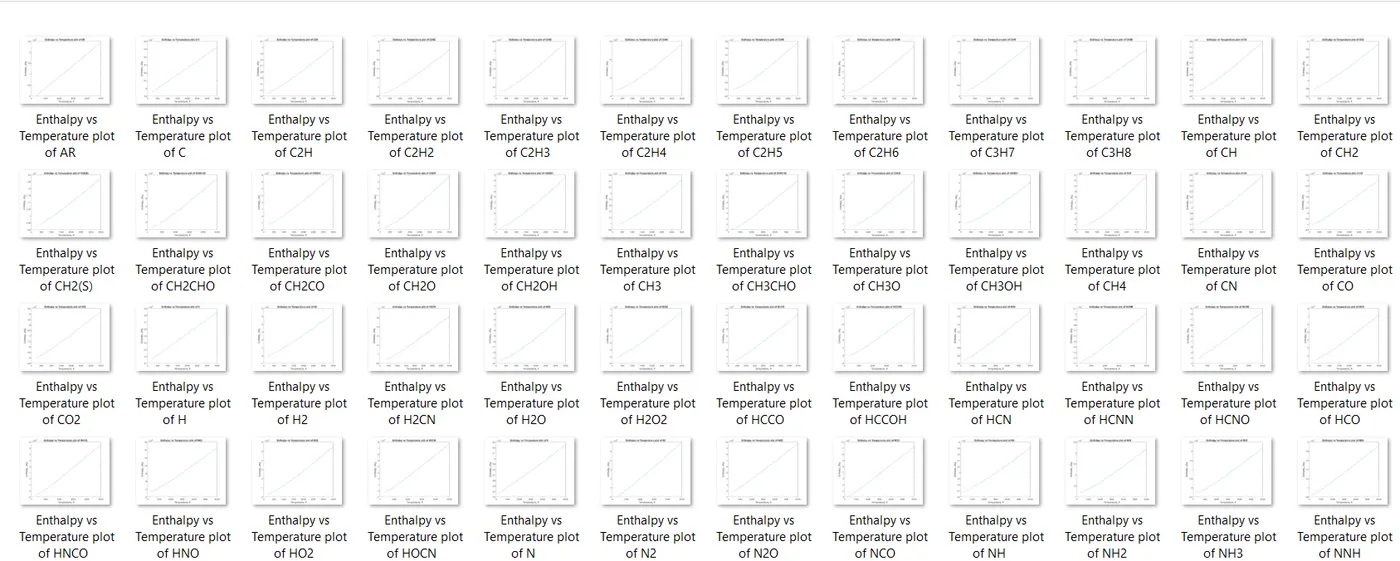
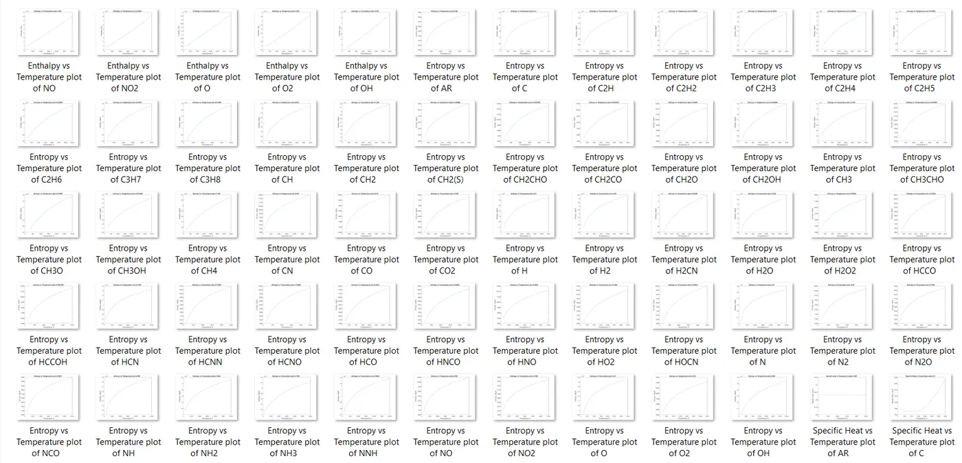
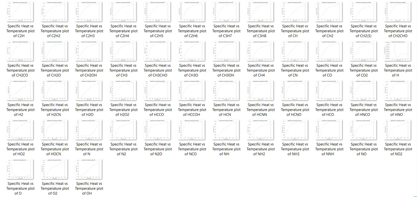
The folder where the plots are saved:
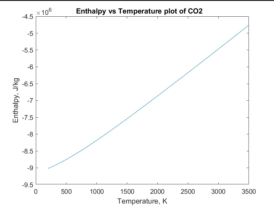
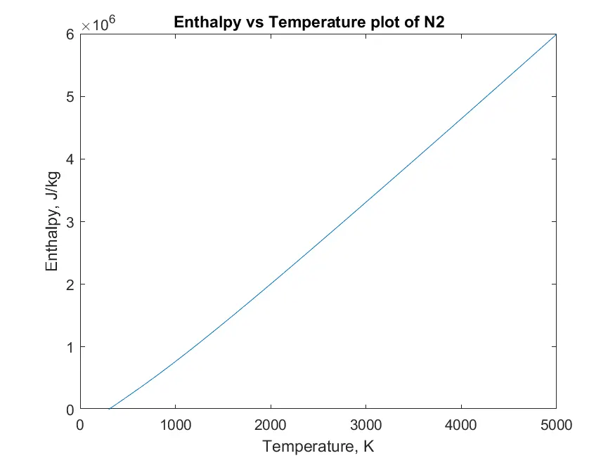
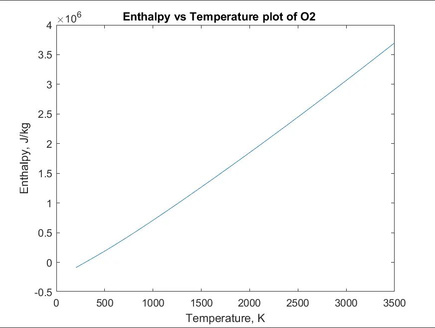
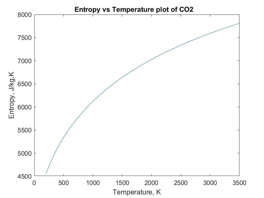
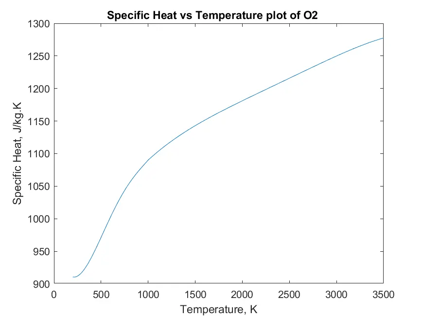
Plots for O2, N2, and CO2: