Project 2 - Rankine cycle Simulator
The Code:
clear all
close all
clc

%% Rankine cycle simulator

fprintf('\n Rankine Cycle:\n')
fprintf(' 1-2 is Isentropic Expansion in Turbine\n')
fprintf(' 2-3 is constant pressure heat removal\n')
fprintf(' 3-4 is Isentropic Compression in Pump \n')
fprintf(' 4-1 Constant pressure Heat addition in Boiler\n\n')

%% Input data
P1=input('Please input pressure at turbine inlet in bars: ');
T1=input('\nPlease input temperature at turbine inlet in degree celcius: ');
P2=input('\nPlease input pressure at turbine outlet in bars: ');
%% Calling data from XSteam file

%For point 1
h1 = XSteam('h_pT', P1, T1);        % Enthaply at pressure and Temperature 1
s1 = XSteam('s_pT', P1, T1);        % Entropy at pressure and Temperature 1
T1_sat= XSteam('Tsat_p', P1);       % saturation temperature at Pressure 1
h1_V= XSteam('hV_p', P1);           % Enthalpy at pressure 1 at vapor phase
h1_L= XSteam('hL_p', P1);           % Enthalpy at pressure 1 at liquid phase
T1_sat_L= XSteam('T_ph', P1,h1_L);  % Saturation temperature 1
s1_sat_L= XSteam('sL_p', P1);       % Entropy at pressure 1 at liquid phase
T1_sat_V= XSteam('T_ph', P1,h1_V);  % Saturation temperature 1
s1_sat_V= XSteam('sV_p', P1);       % Entropy at pressure 1 at vapor phase

%For point 2
s2=s1;                              % Isentropic expansion from 1 to 2
h2 = XSteam('h_ps', P2, s2);        % Enthaply at pressure and Temperature 2
x2= XSteam('vx_ph',P2,h2);          % Vapor volume fraction at 2
W_output=h1-h2;                     % Work output at turbine
Cp2 = XSteam('Cp_ps',P2,s2);        % Specific isobaric heat capacity
Cv2 = XSteam('Cv_ps',P2,s2);        % Specific isochoric heat capacity
k = Cp2/Cv2;
T2 = T1/((P1/P2)^((k-1)/k));        % Temperature at State point 4


%For point 3
P3=P2;                              % constant pressure heat rejection
%since the flow is going into pump next, we want to avoid water vapor enetering the pump, thus the flow should be saturated liquid
s3_L = XSteam('sL_p', P3);          % Saturated liquid entropy at Pressure 3
s3_V = XSteam('sV_p', P3);          % Saturated vapor entropy at pressure 3
h3 = XSteam('hL_p', P3);            % Saturated liquid Enthalpy at Pressure 3
T3= XSteam('T_ph', P3, h3);         % Temperature at 3
T3_sat= XSteam('Tsat_p', P3);       % Saturation temperature at 3
x3= XSteam('vx_ph',P3,h3);          % Vapor volume fraction at 3
Qdot_out=h2-h3;                     % Heat rejected at constant pressure from the system

%for point 2
if s2>=s3_V && T2>=T3_sat
Cp2 = XSteam('Cp_ps',P2,s2);        % Specific isobaric heat capacity
Cv2 = XSteam('Cv_ps',P2,s2);        % Specific isochoric heat capacity
k = Cp2/Cv2;
T2 = T1/((P1/P2)^((k-1)/k));        % Temperature at State point 4
else
T2prime=XSteam('T_ps',P2,s2);       % the temperature at which the inlet temperature to condensor should reach, inorder to go through the isobaric process at P2
end

%For point 4
s4=s3_L;                            % Isentropic compression from 3 to 4
P4=P1;                              % Constant pressure heat addition
h4 = XSteam('h_ps', P4, s4);        % Enthalpy at pressure and entropy 4

Cp4 = XSteam('Cp_ps',P4,s4);        % Specific isobaric heat capacity
Cv4 = XSteam('Cv_ps',P4,s4);        % Specific isochoric heat capacity
k = Cp4/Cv4;
T4 = T3/((P3/P4)^((k-1)/k));        % Temperature at State point 4 (isentropic relations)

x4= XSteam('vx_ph',P4,h4);          % Vapor volume fraction at 4
W_input=h4-h3;                      % Work done by pump
Qdot_in=h1-h4;                      % Heat added at constant pressure to the system


%% Calculations

%Net work done
W_net=W_output-W_input;             % Net work produced by system

%Thermal Efficiency of Rankine Cycle
T_eff = (W_net/Qdot_in)*100;

%Back work ratio
Back_work_ratio=W_input/W_output;   % amount of work taken from the output by the pump

%% Plotting

%Plotting for Saturation Line
T = linspace(1,400,1000);
for i = 1:length(T)
    sL(i) = XSteam('sL_T' ,T(i));   % Saturated Liquid Entropy
    sV(i) = XSteam('sV_T' ,T(i));   % Saturated Vapour Entropy
    hL(i) = XSteam('hL_T' ,T(i));   % Saturated Liquid Enthalpy
    hV(i) = XSteam('hV_T' ,T(i));   % Saturated Vapour Enthalpy
end

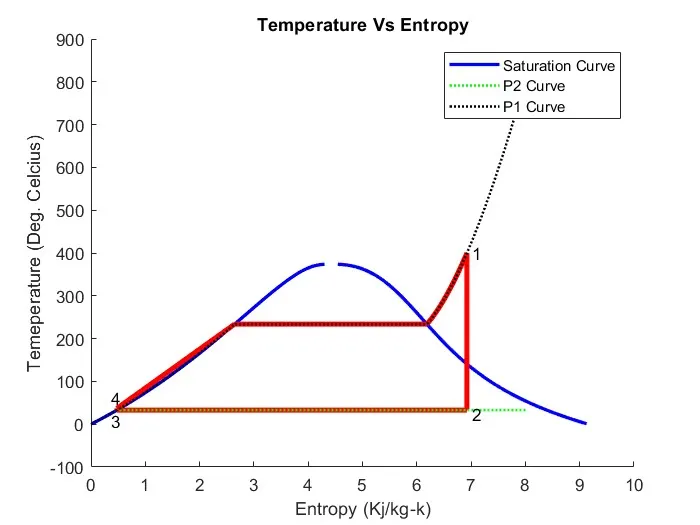
%% Plotting T-S Diagram for Rankine Cycle
figure('Name','T-S Diagram')

if s2>=s3_V && T2>=T3_sat

hold on

plot(sL,T,'color','b','linewidth',2) % plots the liquid saturation entropy curve

plot(sV,T,'color','b','linewidth',2) % plots the vapor saturation entropy curve

plot([s1 s2],[T1 T2], 'color', 'r', 'linewidth',3) % plots the isentropic expansion process s1 and s2 are equal

T2prime=XSteam('T_ps',P2,s2); % the temperature at which the inlet temperature to condensor should reach, inorder to go through the isobaric process at P2

plot([s2 s2],[T2 T2prime], 'color', 'r', 'linewidth',3)

plot([s3_V s3_L],[T3_sat T3_sat], 'color', 'r', 'linewidth',3) % plots the isobaric heat rejection process inside
% the curve where temperature remains the same at saturation temperature T3_sat and entropy decreases until it reaches entropy of saturated liquid

plot([s3_L s4],[T3_sat T4], 'color', 'r', 'linewidth',3) % plots the isentropic compression process where pressure and temperature increases

plot([s4 s1_sat_L],[T4 T1_sat_L], 'color', 'r', 'linewidth',3) % Constant pressure heat addition till saturation temperature is achieved

plot([s1_sat_L s1_sat_V],[T1_sat_L T1_sat_V], 'color', 'r', 'linewidth',3) % Constant pressure heat addition until all liquid converted to vapor phase

% to plot the T-S diagram while heating the vapor till it reaches entropy 1
s_1 = linspace(s1_sat_V,s1,1000); % Entropy range from saturated vapor phase until entropy at 1
for j = 1:length(s_1)
    Tc(j) = XSteam('T_ps',P1,s_1(j)); % Temeprature range corresponding to the entropy values
end
plot(s_1,Tc,'color','r','linewidth',3)

% constant pressure heat rejection until it reaches saturation temperature from 2 to 3
s_2 = linspace(s3_V,s2,200); % Entropy range from s2 til saturated vapor entropy at 3
for j = 1:length(s_2)
    Tk(j) = XSteam('T_ps',P2,s_2(j)); % Temperature range corresponding to entropy values
end
plot(s_2,Tk,'color','r','linewidth',3)


% To visualize the constant pressure T-S line for Pressure 2
sp2=linspace(0,8,1000);
for j = 1:length(sp2)
    Ts(j) = XSteam('T_ps',P2,sp2(j));
end
plot(sp2,Ts,'color','g','linewidth',1.5, 'LineStyle',':')

% To visualize the constant pressure T-S line for Pressure 1
sp1=linspace(0,8,1000);
for j = 1:length(sp1)
    Ts(j) = XSteam('T_ps',P1,sp1(j));
end
plot(sp1,Ts,'color','k','linewidth',1.5, 'LineStyle',':')

text(s1+0.1, T1, '1')
text(s2+0.1, T2-10, '2')
text(s3_L-0.1, T3-25, '3')
text(s4-0.1, T4+25, '4')

title('Temperature Vs Entropy')
xlabel('Entropy (Kj/kg-k)')
ylabel('Temeperature (Deg. Celcius)')
legend('Saturation Curve','','','','','','','','','','P2 Curve','P1 Curve')

else
hold on

plot(sL,T,'color','b','linewidth',2) % plots the liquid saturation entropy curve

plot(sV,T,'color','b','linewidth',2) % plots the vapor saturation entropy curve

plot([s1 s2],[T1 T2prime], 'color', 'r', 'linewidth',3) % plots the isentropic expansion process s1 and s2 are equal

plot([s2 s3_L],[T2prime T3_sat], 'color', 'r', 'linewidth',3) % plots the isobaric heat rejection process inside
% the curve where temperature remains the same at saturation temperature T3_sat and entropy decreases until it reaches entropy of saturated liquid

plot([s3_L s4],[T3_sat T4], 'color', 'r', 'linewidth',3) % plots the isentropic compression process where pressure and temperature increases

plot([s4 s1_sat_L],[T4 T1_sat_L], 'color', 'r', 'linewidth',3) % Constant pressure heat addition till saturation temperature is achieved

plot([s1_sat_L s1_sat_V],[T1_sat_L T1_sat_V], 'color', 'r', 'linewidth',3) % Constant pressure heat addition until all liquid converted to vapor phase

% to plot the T-S diagram while heating the vapor till it reaches entropy 1
s_1 = linspace(s1_sat_V,s1,1000); % Entropy range from saturated vapor phase until entropy at 1
for j = 1:length(s_1)
    Tc(j) = XSteam('T_ps',P1,s_1(j)); % Temeprature range corresponding to the entropy values
end
plot(s_1,Tc,'color','r','linewidth',3)

% To visualize the constant pressure T-S line for Pressure 2
sp2=linspace(0,8,1000);
for j = 1:length(sp2)
    Ts(j) = XSteam('T_ps',P2,sp2(j));
end
plot(sp2,Ts,'color','g','linewidth',1.5, 'LineStyle',':')

% To visualize the constant pressure T-S line for Pressure 1
sp1=linspace(0,8,1000);
for j = 1:length(sp1)
    Ts(j) = XSteam('T_ps',P1,sp1(j));
end
plot(sp1,Ts,'color','k','linewidth',1.5, 'LineStyle',':')

text(s1+0.1, T1, '1')
text(s2+0.1, T2prime-10, '2')
text(s3_L-0.1, T3-25, '3')
text(s4-0.1, T4+25, '4')

title('Temperature Vs Entropy')
xlabel('Entropy (Kj/kg-k)')
ylabel('Temeperature (Deg. Celcius)')
legend('Saturation Curve','','','','','','','','P2 Curve','P1 Curve')

end

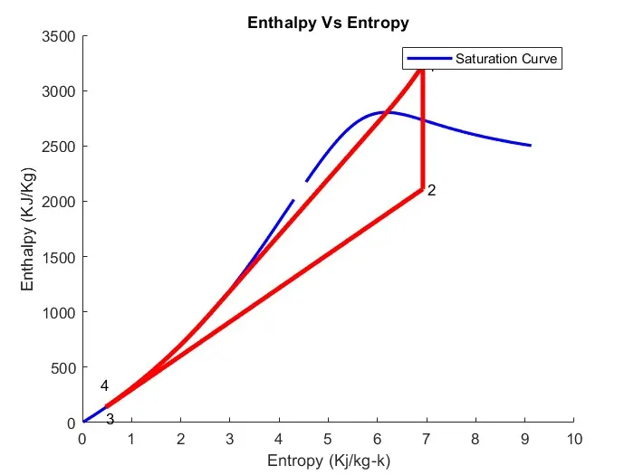
%% Plotting H-S diagram
figure('Name','H-S Diagram')
hold on
plot(sL,hL,'color','b','linewidth',2)
plot(sV,hV,'color','b','linewidth',2)

%Isentropic expansion process
plot([s1 s2],[h1 h2],'color','r','linewidth',3)

% Constant pressure process of heat removal until saturated liquid is achieved
% therefore from h2 to h3 at liquid phase at constant p2
h3_L=XSteam('hL_p',P3); % end point
h23 = linspace(h2,h3_L,1000); %from h2 to h3_L
for i = 1:length(h23)
    s23(i) = XSteam('s_ph',P2,h23(i)); % since at constant pressure p2
end
plot(s23,h23,'color','r','linewidth',3)


% isentropic compression process
plot([s3_L s4],[h3_L h4], 'color', 'r', 'linewidth',3)

% Constant pressure process of heat addition until saturated vapor is achieved
% therefore from h4 to h1 at vapor phase at constant p1
h41 = linspace(h4,h1,1000); %from h4 to h1
for i = 1:length(h41)
    s41(i) = XSteam('s_ph',P1,h41(i));  % since at constant pressure p1
end
plot(s41,h41,'color','r','linewidth',3)

text(s1+0.1,h1,'1')
text(s2+0.1,h2,'2')
text(s3_L,h3-100,'3')
text(s4-0.1,h4+200,'4')
title('Enthalpy Vs Entropy')
xlabel('Entropy (Kj/kg-k)')
ylabel('Enthalpy (KJ/Kg)')
legend('Saturation Curve')

%% Displaying Results in Command window
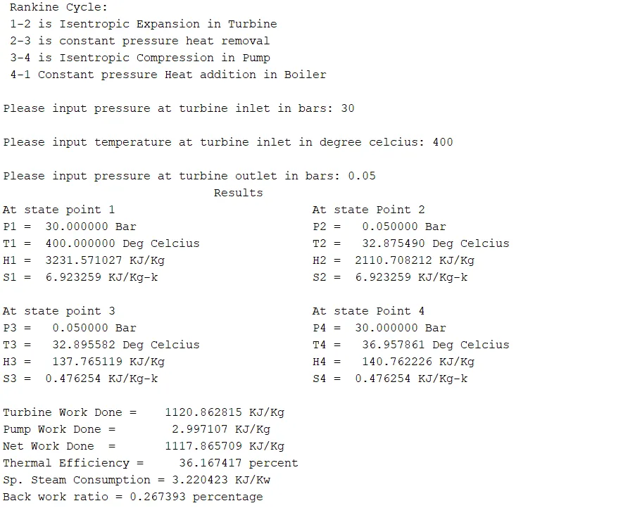
disp('                              Results')
fprintf('At state point 1\t\t\t\t\t\t\t')
fprintf('At state Point 2\n')
fprintf('P1 = %10f Bar\t\t\t\t\t\t\t',P1);
fprintf('P2 = %10f Bar\n',P2);
fprintf('T1 = %11f Deg Celcius\t\t\t\t',T1);
fprintf('T2 = %11f Deg Celcius\n',T2prime);
fprintf('H1 = %12f KJ/Kg\t\t\t\t\t\t',h1);
fprintf('H2 = %12f KJ/Kg\n',h2);
fprintf('S1 = %9f KJ/Kg-k\t\t\t\t\t\t',s1);
fprintf('S2 = %9f KJ/Kg-k\n',s2);
fprintf('\n')
fprintf('At state point 3\t\t\t\t\t\t\t')
fprintf('At state Point 4\n')
fprintf('P3 = %10f Bar\t\t\t\t\t\t\t',P3);
fprintf('P4 = %10f Bar\n',P4);
fprintf('T3 = %11f Deg Celcius\t\t\t\t',T3);
fprintf('T4 = %11f Deg Celcius\n',T4);
fprintf('H3 = %12f KJ/Kg\t\t\t\t\t\t',h3);
fprintf('H4 = %12f KJ/Kg\n',h4);
fprintf('S3 = %9f KJ/Kg-k\t\t\t\t\t\t',s3_L);
fprintf('S4 = %9f KJ/Kg-k\n',s4);
fprintf('\n')
fprintf('Turbine Work Done = %14f KJ/Kg\n',W_output)
fprintf('Pump Work Done = %15f KJ/Kg\n',W_input)
fprintf('Net Work Done  = %17f KJ/Kg\n',W_net)
fprintf('Thermal Efficiency = %13f percent\n',T_eff)
fprintf('Sp. Steam Consumption = %f KJ/Kw\n',3600/W_net)
fprintf('Back work ratio = %f percentage\n',(W_input/W_output)*100)
The Plots:
Command window screenshot: