Week 5 - Genetic Algorithm

GENETIC ALGORITHM:

 Genetic Algorithm is an algorithm used to find the global minima of a given problem in matlab. It is an optimization tool available in matlab and many other platforms.

The genetic algorithm is a type of optimization algorithm inspired by the natural process of selection and genetics. It is used in computer science and engineering to find approximate solutions to complex search and optimization problems. Genetic algorithms are part of a broader class of algorithms known as evolutionary algorithms.

The basic idea behind a genetic algorithm is to evolve a population of potential solutions to a problem over multiple generations, gradually improving the quality of the solutions, as they begin to converge to single solution (the best one).

The steps involved in Genetic Algorithm are:

Initialization: A population of potential (within the bounds specified) solutions, often represented as a set of chromosomes (usually strings of binary or numerical values), is created randomly.

Evaluation: Each solution in the population is evaluated using a fitness function that measures how well each solution solves the problem.

Selection: Solutions are selected for reproduction based on their fitness values. Solutions with higher fitness values have a higher chance of being selected. This mimics the idea that better solutions are more likely to pass their genetic information to the next generation.

Crossover (Recombination): Pairs of selected solutions (parents) exchange genetic information to create new solutions (offspring). This is analogous to genetic recombination in sexual reproduction.

Mutation: Occasionally, some parts of the offspring's genetic information are randomly altered. Mutation introduces diversity into the population, ensuring exploration of new regions in the search space.

Replacement: The new offspring replaces some of the less fit members of the current population, ensuring that the population size remains constant.

Termination: The algorithm iterates through the selection, crossover, mutation, and replacement steps for a specified number of generations or until a termination condition is met, such as finding a satisfactory solution or reaching a time limit.

Genetic algorithms are useful for solving complex optimization problems with many possible solutions. They are applied in various fields, including engineering, economics, biology, and machine learning, where finding an optimal or near-optimal solution is challenging or where the solution space is not well-understood. By mimicking the principles of evolution, genetic algorithms can efficiently search large solution spaces and discover high-quality solutions.

THE SYNTAX:

[x,Fval,exitFlag,Output] = = ga(@FitnessFunction,numberOfVariables,[],[],[],[],[0 0],[0.6 0.6],[],opts);

exitflag - an integer identifying the reason the algorithm terminated.
x - the x and y values where minimum is obtained.
fval- the minimum function value.
output - a structure that contains output from each generation and other information about the performance of the algorithm.
FitnessFunction - the function used, in our case, stalagmite function.
numberOfVariables - the number of variables, in our case 2 (x and y).
The empty brackets are A,B,Aeq,Beq respectively which are of no use to us. These are used incase of linear inequalities.
[0 0] and [0.6 0.6] are lower and upper bounds respectivvely. [0 0] corresponds to [lower_bound_of_x_values lower_bound_of_y_values] and [0.6 0.6] corresponds to [upper_bound_of_x_values upper_bound_of_y_values].

FUCNTIONS:

STALAGMITE:

function [f]= stalagmite(z)

% the stalagmite function is created as per the formulae shown in the video

f1x= (sin((5.1*pi()*z(1)) + 0.5))^6;

f1y= (sin((5.1*pi()*z(2)) + 0.5))^6;

f2x= exp(-4*log(2)*((z(1)-0.0667)^2)/0.64);

f2y= exp(-4*log(2)*((z(2)-0.0667)^2)/0.64);

f=f1x*f2x*f1y*f2y;

end

FLIPPED_STALAGMITE:

function [f]= flipped_stalagmite(z)

%the negative value of stalagmite function is found so that the actual maximum value of stalagmite becomes the minimum

f=-1*stalagmite(z);

end

ACTUAL CODE:

clear all
close all
clc

%% the function is plotted for x and y values between 0 and 0.6
x=linspace(0,0.6,150); %creates 150 values for x equally spaced between 0 and 0.6
y=linspace(0,0.6,150); %creates 150 values for y equally spaced between 0 and 0.6

%% to find and plot the stalagmite function for each values of x and y
%generating 2D mesh from where each and every combination of x and y values can be obtained
[xx yy]= meshgrid(x,y);

%evaluating stalagmite function:

for i=1: length(xx)
    for j= 1: length(yy)
        input_vector(1)=xx(i,j); % x entry for the stalagmite function
        input_vector(2)=yy(i,j); % y entry for the stalagmite function
        f(i,j)= stalagmite(input_vector); % evaluates the stalagmite function for the corresponding combination of x and y values
    end
end

surfc(xx,yy,f); %creates 3D plot to visualize the stalagmite function
xlabel('x value'); %to label the x axis
ylabel('y value'); %to label the y axis
shading interp %to change the grid lines into shading of style 'interp'

%% To find the maximum value of the stalagmite function using Genetic Algorithm

% the setup of genetic algorithm

%to set up the following options
%the line below lets us plot the function vlaues versus no.of iteraations and also the max number of iterations is kept to 200, since the poblem converge fast
opts = optimoptions(@ga,'PlotFcn',@gaplotbestf,'MaxGenerations',200);
opts.PopulationSize=70; % initial population size, the more the size, the more the computation time, the more accurate in most cases
opts.InitialPopulationRange=[0 0.6; 0 0.6]; %initial population created within the region

%the x and y values at which the function value is minimum is obtained, the minimum function value is also obtained
%x_y_values are the x and y values and f_val is the minimum function value
%instead of stalagmite function, flipped_stalagmite is used, which multiplies the stalagmite function with -1 to get negative values
%therefore the maximum value will be the minimum in flipped_stalagmite, but the x_y_values will be the same
%the empty brackets are necessary according to the syntax of ga
[x_y_values,f_val,exitflag,output] = ga(@flipped_stalagmite, 2, [], [], [], [], [0 0], [0.6 0.6],[],opts); % [0 0] & [0.6 0.6] are lower and upper bounds respectively, only x and y values wihtin the bounds be considered

%% to print out the final answers
fprintf('The maximum value of stalagmite function is obtained at %0.4f x value and %0.4f y value\n',x_y_values(1),x_y_values(2))
fprintf('The maximum value of stalagmite function is %0.3f\n',stalagmite(x_y_values))
fprintf('the number of iterations taken to converge is %d\n',output.generations) %output is a structure and one of the elements in it gives us the number of generations

SCREENSHOTS:

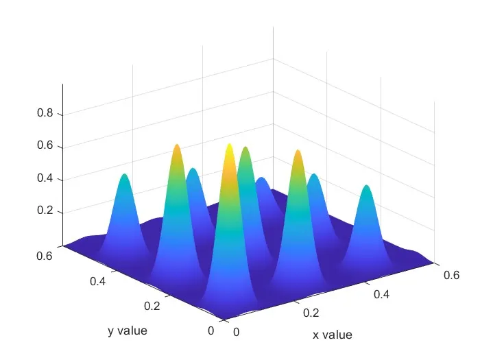
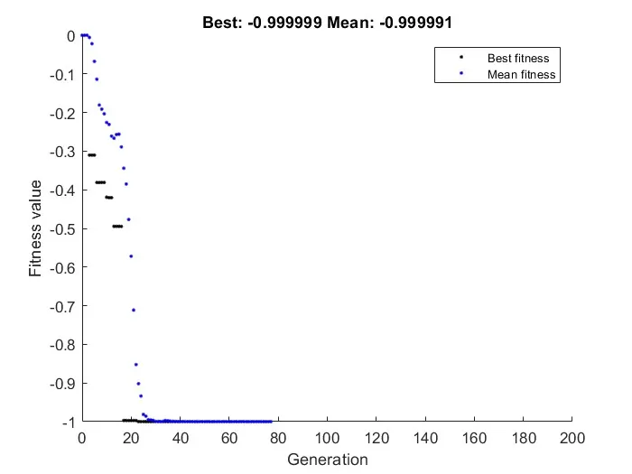
The above plot is for flipped_stalagmite which is basically the negative values of stalagmite function.

Therefore the actual global maximum value of the stalagmite function will be 1.

SOLUTIONS PRINTED AT COMMAND WINDOW:

The maximum value of stalagmite function is obtained at 0.0668 x value and 0.0668 y value

The maximum value of stalagmite function is 1.000

the number of iterations taken to converge is 77

ERROR FACED:

Sometimes the global minimum is not obtained as the value converges to a local minimum. But this occurs rarely.

REFERENCE:

https://www.mathworks.com/help/gads/options-in-genetic-algorithm.html

https://en.wikipedia.org/wiki/Genetic_algorithm

https://www.mathworks.com/help/gads/what-is-the-genetic-algorithm.html