Project-1: Modelling an electric Car with Li-ion battery
Aim:-
Create a MATLAB model of electric car which uses lithium ion battery and suitable motor. Choose suitable blocks from Simscape or Powertrain block set. Implement the vehicle speed control using PI controller and generate brake and accelerator commands. Avoid using readymade driver block for speed control.
Prepare a report about your model including following:
Objectives, System level configurations, Model parameters, Results, Conclusion.
(Note- The simulink model file should be compulsorily attached)
Answer:-
Objectives:-To design the Li-Ion battery based electric car.
Power calculation:-
Note:- By using excel calculator we can calculate the power requirement of a particular vehicle.
As we will change the mass,area, driving condition(hill or flat surface) and other parameters, the ratings will vary. and from this calculation we can do analysis for power requirement for the car for various driving condiciton.
| Vehicle Power Requirement Calculations | ||||||||
| Electric CAR_Li-ION | ||||||||
| Rolling resistance calculation | ||||||||
| Kerb weight(kg) | 500 | |||||||
| Payload(kg) | 0 | Pay load on the pessanger inside the car) | ||||||
| Coefficient of rolling resistance | 0.015 | |||||||
| Rolling resistance force(N) | 73.575 | (coefficient of rolling resistance*(kerb weight+payload)*g | RR force+air drag force=tractive force | |||||
| Air Drag Calculation | power= tractiveforce*velocity(m/s) | |||||||
| Air Desnsity(kg/m3) | 1.25 | |||||||
| Width(m) | 2 | |||||||
| Height(m) | 2 | |||||||
| Frontal Area(m2) | 4 | |||||||
| Drag Coefficient | 0.33 | |||||||
| Speed(kmph) | 60 | Top speed is 55kmph | ||||||
| Velocity(m/s) | 16.66666667 | |||||||
| Air Drag Force(N) | 229.1666667 | (air density*frontal area*drag coefficient*velocity^2) | convert speed from kmph to m/s | |||||
| Total power(rolling+air drag) | 5045.694444 | (rolling resistance force+Air drag force)*velocity | ||||||
| Hill Climbing calculation | ||||||||
| Angle(degrees) | 10 | |||||||
| Angle(radians) | 0.174444444 | |||||||
| Speed during hill climbing | 20 | |||||||
| Velocity(m/s) | 5.555555556 | |||||||
| Force(N) | 851.3169034 | (m*g*sin(angle) | ||||||
| Hill vlimbing power(kW) | 4.729538352 | (Force*velocity) | ||||||
| Acceleration Power Calculation | ||||||||
| final speed from 0 to xkmph) | 20 | |||||||
| Velocity(m/s) | 5.555555556 | |||||||
| Acceleration time(sec) | 2.3 | 643.0041152 | ||||||
| Acceleration(m/s2) | 2.415458937 | (a=velocity/acceleration time) | ||||||
| Acceleration force(N) | 6709.608159 | F=m*a*v | ||||||
| Acceleration Power(kW) | 643.0041152 | P=(0.5*m*V^2)/acceleration time | ||||||
| Total Force(N) | 7863.666729 | |||||||
| Total Power(W) | 5693.428098 | |||||||
| Total Power (kW) | 5.693428098 | |||||||
Matlab Model:-
Step1) Designing the Load (Vehicle)
Here the vehicle is considered as a load on motor.
Required blocks to design vehicle are as follows:
1)Tire (Magic Formula)

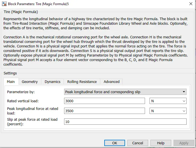
The Tire (Magic Formula) block models a tire with longitudinal behavior given by the Magic Formula [1], an empirical equation based on four fitting coefficients. The block can model tire dynamics under constant or variable pavement conditions.
The longitudinal direction of the tire is the same as its direction of motion as it rolls on pavement. This block is a structural component based on the Tire road interaction block.
To increase the fidelity of the tire model, you can specify properties such as tire compliance, inertia, and rolling resistance. However, these properties increase the complexity of the tire model and can slow down simulation. Consider ignoring tire compliance and inertia if simulating the model in real time or if preparing the model for hardware-in-the-loop (HIL) simulation.
Tire Model
The Tire (Magic Formula) block models the tire as a rigid wheel-tire combination in contact with the road and subject to slip. When torque is applied to the wheel axle, the tire pushes on the ground (while subject to contact friction) and transfers the resulting reaction as a force back on the wheel. This action pushes the wheel forward or backward. If you include the optional tire compliance, the tire also flexibly deforms under load.
The figure shows the forces acting on the tire. The table defines the tire model variables.
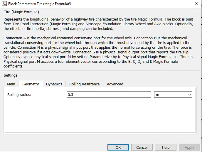
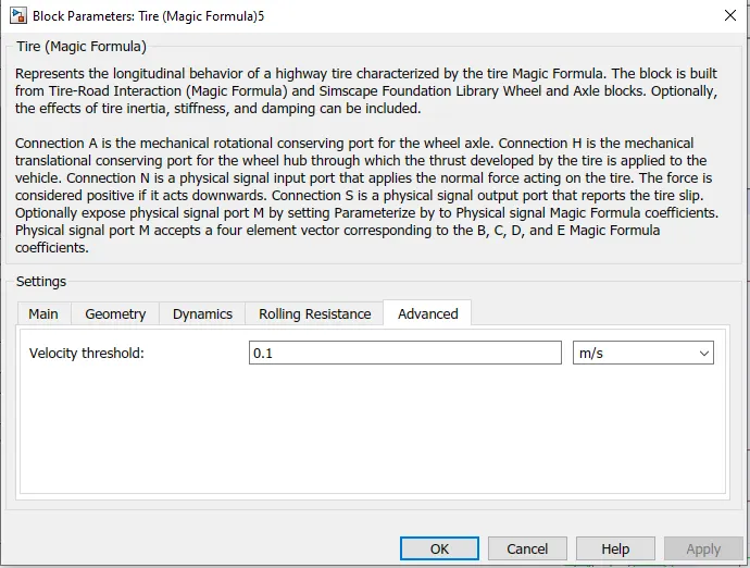
Parameter Settings:-
2)PS Terminator

Use the PS Terminator block to cap physical signal output ports that do not connect to other blocks
3)PS Constant

The PS Constant block generates a physical signal of a constant value. You specify the value and unit of the signal as the Constant parameter.
4)Vehicle Body
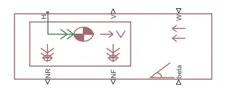
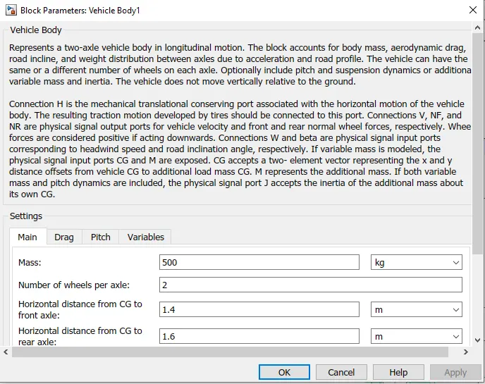
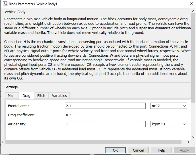
The Vehicle Body block represents a two-axle vehicle body in longitudinal motion. The vehicle can have the same or a different number of wheels on each axle. For example, two wheels on the front axle and one wheel on the rear axle. The vehicle wheels are assumed identical in size. The vehicle can also have a center of gravity (CG) that is at or below the plane of travel.
The block accounts for body mass, aerodynamic drag, road incline, and weight distribution between axles due to acceleration and road profile. Optionally include pitch and suspension dynamics. The vehicle does not move vertically relative to the ground.
The block has an option to include an externally-defined mass and an externally-defined inertia. The mass, inertia, and center of gravity of the vehicle body can vary over the course of simulation in response to system changes.
Model
The vehicle axles are parallel and form a plane. The longitudinal, x, direction lies in this plane and perpendicular to the axles. If the vehicle is traveling on an incline slope, β, the normal, z, direction is not parallel to gravity but is always perpendicular to the axle-longitudinal plane.
This figure and table define the vehicle motion model variables.
Vehicle Dynamics and Motion
Parameter Settings:-
5)Inertia

The Inertia block represents an ideal mechanical translational inertia that is described with the following equation:
T=Jdωdt
where:
-
T is inertia torque.
-
J is inertia.
-
ω is angular velocity.
-
t is time.
6)Simple Gear

The Simple Gear block represents a gearbox that constrains the connected driveline axes of the base gear, B, and the follower gear, F, to corotate with a fixed ratio that you specify. You choose whether the follower axis rotates in the same or opposite direction as the base axis. If they rotate in the same direction, the angular velocity of the follower, ωF, and the angular velocity of the base, ωB, have the same sign. If they rotate in opposite directions, ωF and ωB have opposite signs. You can easily add and remove backlash, faults, and thermal effects.
Matlab Model of Vehicle:-
Step2) DC motor and Conveter
Required blocks to design motor and converter are as follows:
1) DC Motor

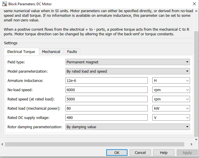
The DC Motor block represents the electrical and torque characteristics of a DC motor using the following equivalent circuit model:
You specify the equivalent circuit parameters for this model when you set the Model parameterization parameter to By equivalent circuit parameters. The resistor R corresponds to the resistance you specify in the Armature resistance parameter. The inductor L corresponds to the inductance you specify in the Armature inductance parameter.
Parameter settings:-
2)H-Bridge
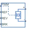
The H-Bridge block represents an H-bridge motor driver. The block has the following two Simulation mode options:
-
PWM— The H-Bridge block output is a controlled voltage that depends on the input signal at the PWM port. If the input signal has a value greater than the Enable threshold voltage parameter value, the H-Bridge block output is on and has a value equal to the value of the Output voltage amplitude parameter. If it has a value less than the Enable threshold voltage parameter value, the block maintains the load circuit using one of the following three Freewheeling mode options:-
Via one semiconductor switch and one freewheeling diode -
Via two freewheeling diodes -
Via two semiconductor switches and one freewheeling diode
The first and third options are sometimes referred to as synchronous operation.
The signal at the REV port determines the polarity of the output. If the value of the signal at the REV port is less than the value of the Reverse threshold voltage parameter, the output has positive polarity; otherwise, it has negative polarity.
-
-
Averaged— This mode has two Load current characteristics options:-
Smoothed -
Unsmoothed or discontinuous
-
Parameter Setting:-
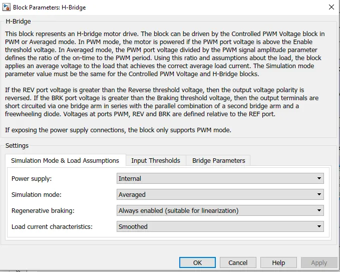
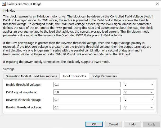
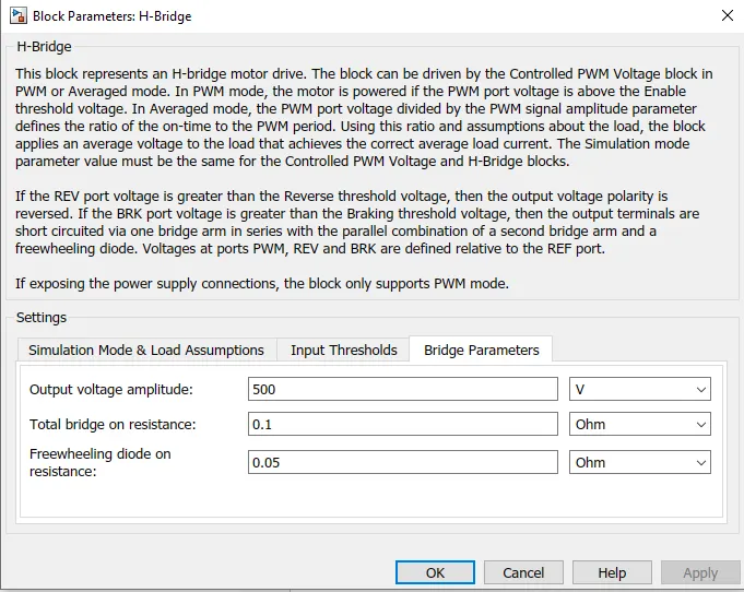
Note:- The H Bridge and Motor ratings are very crucial for any drive to work appropriate and give the desired output. As the motor rating is at 480V, the bridge output volatge should be enough to provide the desired output volatge to the motor. here it is set as 500V. (There will be the switching losses that might occur in power converter because of the switching of the power semiconductor devices).
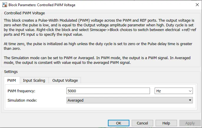
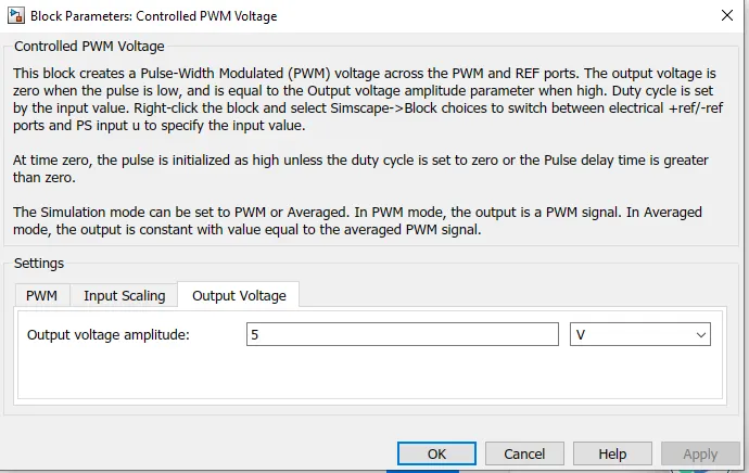
3) Controlled PWM Voltage
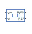
The Controlled PWM Voltage block represents a pulse-width modulated (PWM) voltage source. You can model electrical or physical signal input ports by setting the Modeling option parameter to either:
-
Electrical input ports— The block calculates the duty cycle based on the reference voltage across its ref+ and ref- ports. This option is the default. -
PS input— Specify the duty cycle value directly by using an input physical signal port.
If you set Modeling option to Electrical input ports, the demanded duty cycle is
100∗Vref−VminVmax−Vmin percent
where:
-
Vref is the reference voltage across the ref+ and ref- ports.
-
Vmin is the minimum reference voltage.
-
Vmax is the maximum reference voltage.
Parameter Settings:-
4)Controlled Voltage Source

The Controlled Voltage Source block represents an ideal voltage source that is powerful enough to maintain the specified voltage at its output regardless of the current flowing through the source.
The output voltage is V = Vs, where Vs is the numerical value presented at the physical signal port.
The block has one physical signal input port and two electrical conserving ports associated with its electrical terminals.
5)Current Sensor

The Current Sensor block represents an ideal current sensor, that is, a device that converts current measured in any electrical branch into a physical signal proportional to the current.
Use the + and - ports to connect the sensor in series with the other blocks in the branch where you want to measure the current. Port I outputs the measurement result as a physical signal.
6)Solver Configuration

Each physical network represented by a connected Simscape™ block diagram requires solver settings information for simulation. The Solver Configuration block specifies the solver parameters that your model needs before you can begin simulation.
Each topologically distinct Simscape block diagram requires exactly one Solver Configuration block to be connected to it.
7)Electrical Reference

The Electrical Reference block represents an electrical ground. Electrical conserving ports of all the blocks that are directly connected to ground must be connected to an Electrical Reference block. A model with electrical elements must contain at least one Electrical Reference block.
Matlab Model of DC Motor and Converter:-
Step3) PID Control
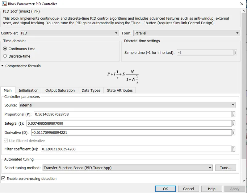
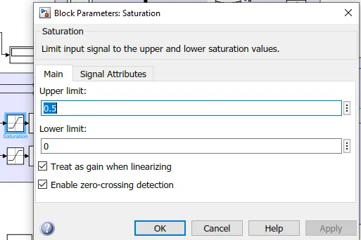
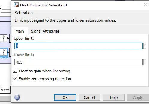
Istead of using the longitude driver block, here we have used PID Controller. By proper tuning of PID controller we can get the proper output speed also the error can be nullified by PID controller. Here to generate acceleration and deceleration command we have used PID controller. The settings are as below:-
Parameter Settings:-
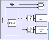
For Acceleration:-
For deceleration:-
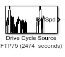
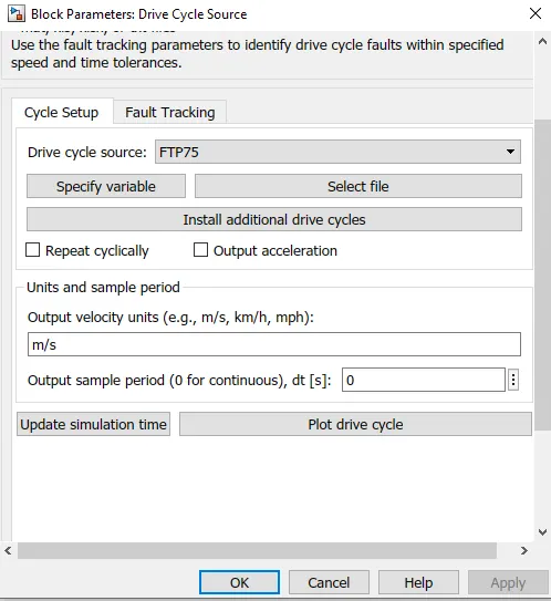
Step4)Drive Cycle
Parameter Settings:-
Step5)Battery SOC
1)Battery
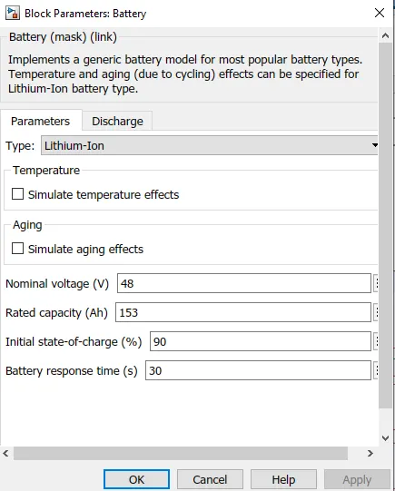
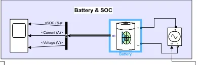
Generally in electric vehicle we are using 48V battery.
Parameters Settings:
2)Controlled Current Source
The Controlled Voltage Source block converts a Simulink® input signal into an equivalent voltage source. The generated voltage is driven by the input signal of the block.
You can initialize the Controlled Voltage Source block with a specific AC or DC voltage. If you want to start the simulation in steady state, the Simulink input must be connected to a signal that begins the simulation as a sinusoidal or DC waveform that corresponds to the initial values.
3)Bus Selector

The Bus Selector block outputs the elements you select from the input bus. The block can output the selected elements separately or in a new virtual bus.
The Bus Selector block does not support mixing message and signal elements as outputs.
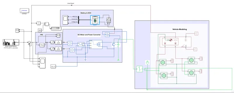
The Overall System:-
Result and Discussion:-
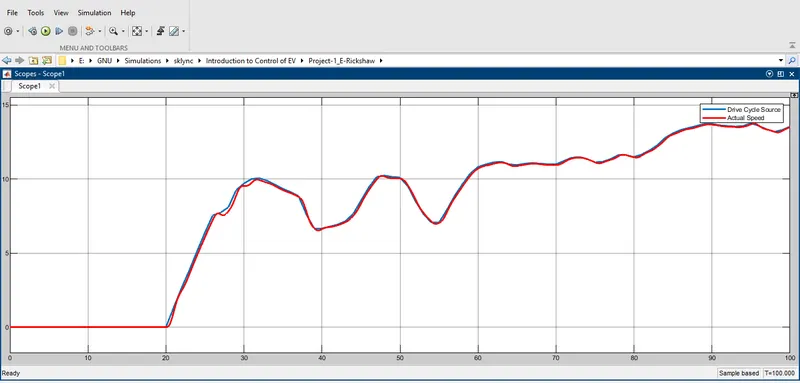
Reference and Actual Speed:-
In below figure we can observe that the reference signal is followed by the actual speed of vehicle by proper tuning of PID controller.
Below figure gives idea about reference speed, actual speed, error signal and PID output.
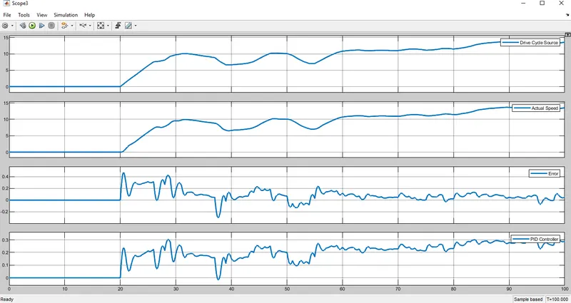
The main roll of PID controller is to correct the error signal. Error signal is generated from the comparision of reference speed and actual vehicle speed. For example the actual speed is 1450RPM and the reference speed is 1500RPM, so the error speed will be 50RPM. Now controller will generate command in such a way that the converter will generate more current so that this 50 rpm will be corrected and the motor will run again on 1500 RPM and the error will be corrected(Vehicle is coupled with the motor as load).
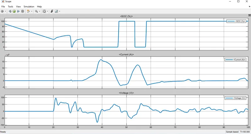
Battery SOC, Current and Voltage:-
Conclusion:-
Here we have simulated the lithium-ion CAR with PID controller. The PID controller is very important for the better performance of any drive system. PID controller will enhance your output by proper tuning. The tuning can be by choosing the apropriate gain for PID and also in MATLAB we can automatically tune the PID parameters. Here we can observe that the actual speed of the vehicle is follwoing the reference speed and the last graph shows the error signal and PID output which corrects the actual speed as per the reference by giving proper command and generates the gate pulses for h-bridge so the particulat power semiconductor device can be switched on anf switched off in required paoportion and the motor will correct its speed and the vehcile can follow the reference speed.