Project-1: Modelling an electric Car with Li-ion battery

Objective:

• Create a MATLAB model of electric car which uses lithium ion battery and suitable motor.
• Implement the vehicle speed control using PI controller and generate brake and accelerator commands.
• For any three standard driving cycles show Energy consumption, Temperature rise of motor and controller.
• Battery State of Charge (SOC) for all the cases.

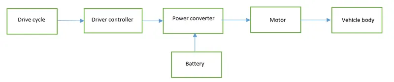
Basic components of Powertrain are,

1. Battery
2. Motor
3. Controller
4. Transmission system
5. Vehicle body

Design in Simulink:

Assumptions:

• Rear wheel driven
• PM brushed type DC motor
• Drive cycles

Procedure:

• Drive Cycle:

Blocks used

Drive cycle

Multiport switch

First choose the Drive cycle which the vehicle will follow. Maximum speed achieved in that drive cycle will decide the design parameters for the motor. Drive cycles taken here are FTP75, Wide open throttle (WOT), Custom data set drive cycle and a contant 45Km/Hr. A multiport switch decides which drive cycle to operate.

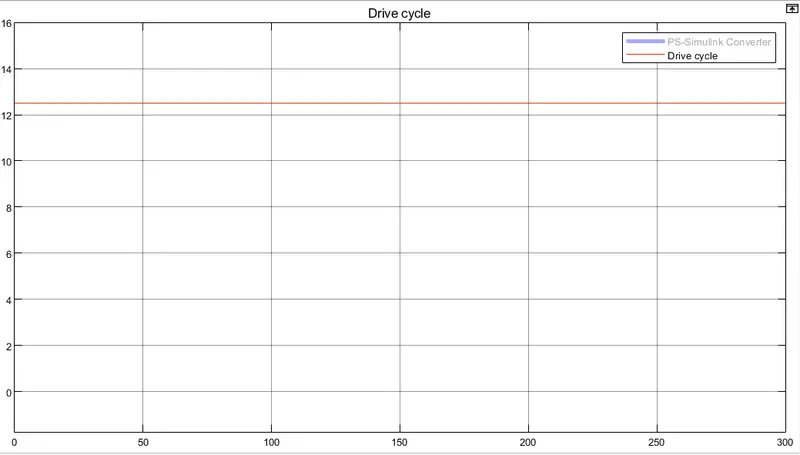
Figure-1 Constant 12.5m/s Drive cycle

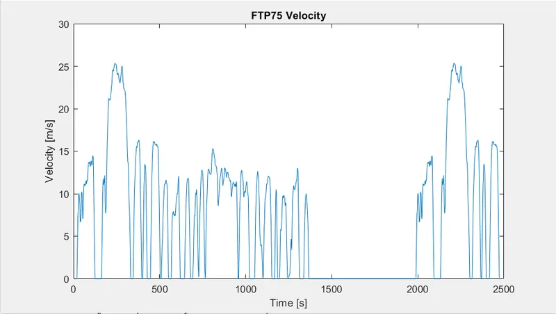
Figure-2 FTP75 Drive cycle

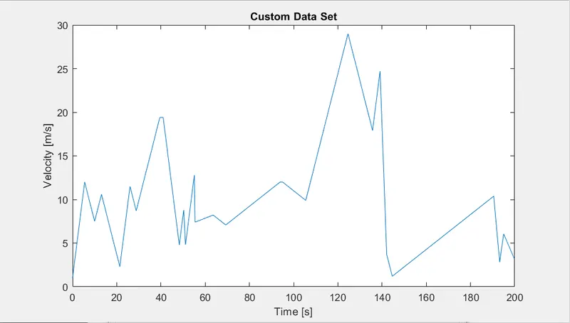
Figure-3 Custom data set

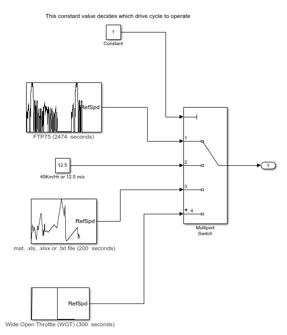
Figure-4 Simulink blockset for input drive cycles

• Vehicle Dynamics

Blocks used

Vehicle body

Simple gear

Tire (Magic)

Rotational Free End

PS Terminator

PS constant

After getting an idea about the maximum speed from the drive cycle, we calculate the Traction force required,

Ft = Traction force = Aerodynamic drag force + Rolling resistance force + Hill climbing force + Acceleration force

Road inclination angle (beta) is considered 0 by using PS constant block and giving value 0. Therefore hill climbing force is 0. Wind velocity (w) is also considered 0

Aerodynamic drag force = Fd = 0.5*(density of air)*(Frontal area)*(Coefficient of drag)*(Velocity^2)

Rolling resistance force = Fr = (Coefficient of rolling resistance)*(weight of vehicle)

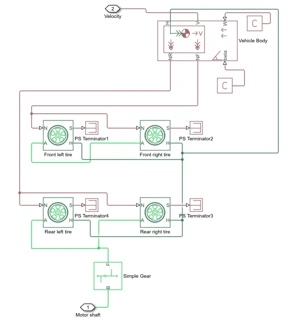
Figure-5 Vehicle dynamics blockset

Using Vehicle body block, we can give the mass, drag and C.G values. Pitch is not considered. Connections V, NF, and NR are physical signal output ports for vehicle velocity and front and rear normal wheel forces, respectively. Connection H is the mechanical translational conserving port associated with the horizontal motion of the vehicle body

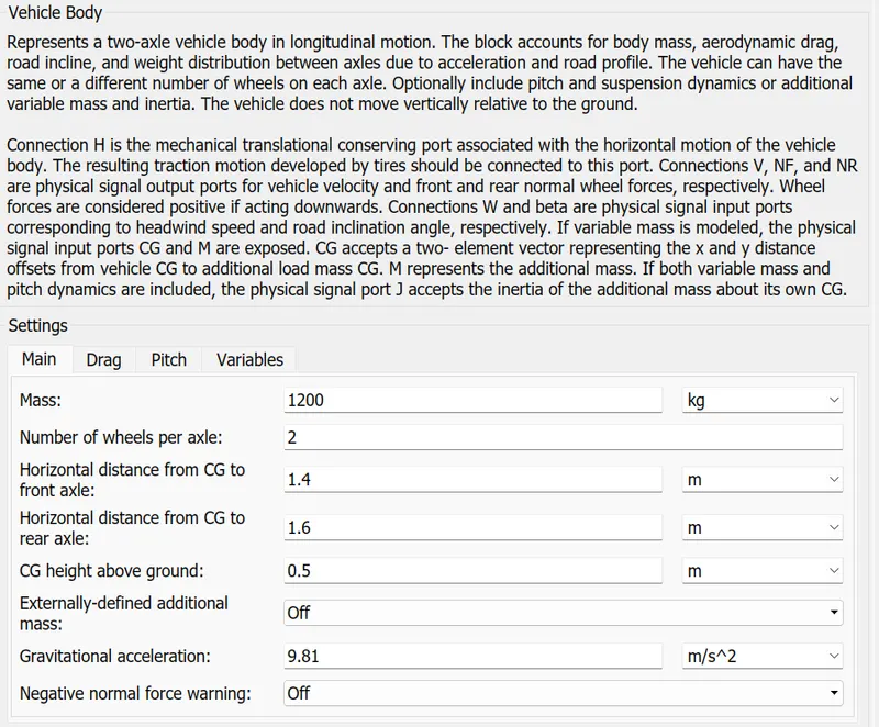
Figure-6 Mass and C.G values of the body

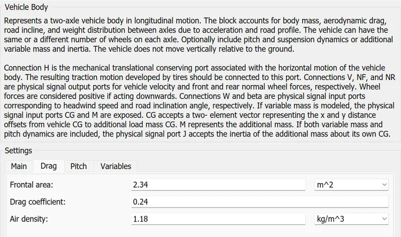
Figure-7 Drag values

Using Tire (magical), We can give the radius of the tire, Rolling resistance coefficients and Longitudnal force acting on it. Connection A is the mechanical rotational conserving port for the wheel axle. Connection H is the mechanical translational conserving port for the wheel hub through which the thrust developed by the tire is applied to the vehicle. Connection N is a physical signal input port that applies the normal force acting on the tire. The force is considered positive if it acts downwards. Connection S is a physical signal output port that reports the tire slip. Dynamics is not considered.

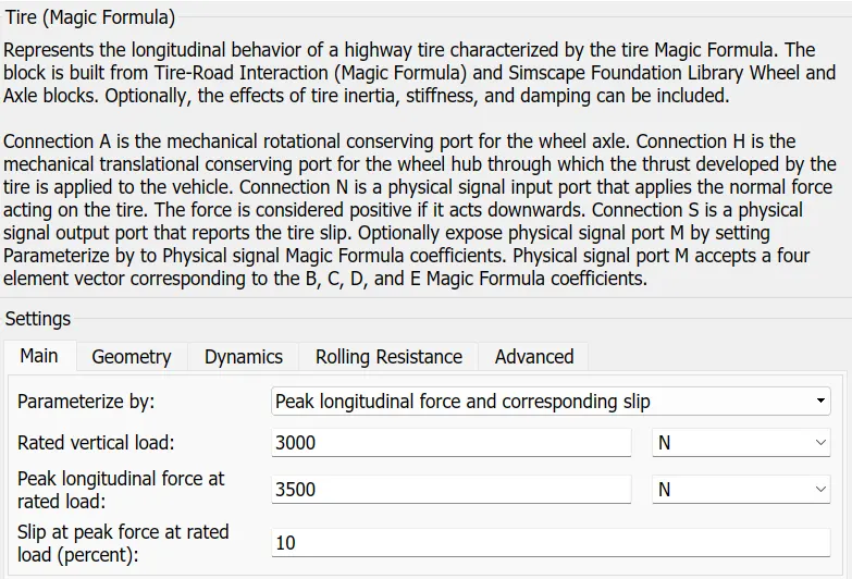
Figure-8 Tire peak longitudnal force

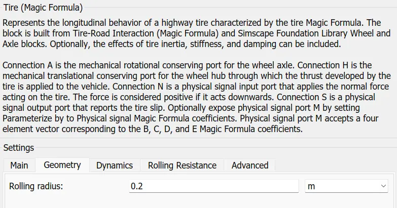
Figure-9 Tire radius

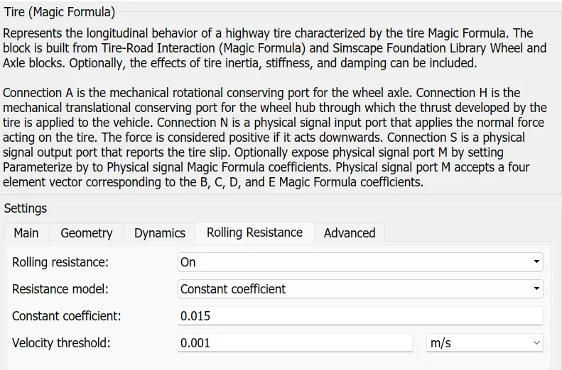
Figure-10 Tire coefficient of rolling resistance

Simple gear box is used with a gear ratio of 8. Cnnection B is connected to the motor shaft and Connection F is connected to rear axle because its a rear wheel drive system.

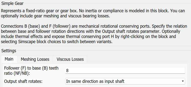
Figure-11 Gear ratio

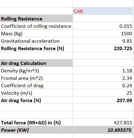
Figure-12 Forces calculation

• Motor and its Controller

Blocks used

Controlled voltage source

Controlled PWM voltage

H-Bridge with thermal port

DC motor with thermal port

Temperature sensor

Current sensor

Electrical, Mechanical and Thermal referance

Maximum velocity (V) from drive cycle taken is 27.7 m/s

V = (pi*diameter of tire * rpm of tire)/60

N = rpm of tire = 1313

Nm = rated rpm = Gear ratio * N = 10580

if speed regulation is 15%, No load rpm = 11500

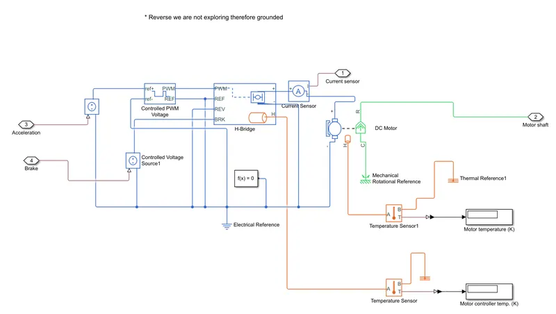
Figure-13 Motor and its controller blockset

Dc motor to be considered is PM brushed type motor. After calculating the Traction power of the wheel, slip and efficiencies are considered and finally mechanical power of the DC motor is calculated. Similarly using whel rpm and speed regulation, motor rated speed and no load speed can be calculated.

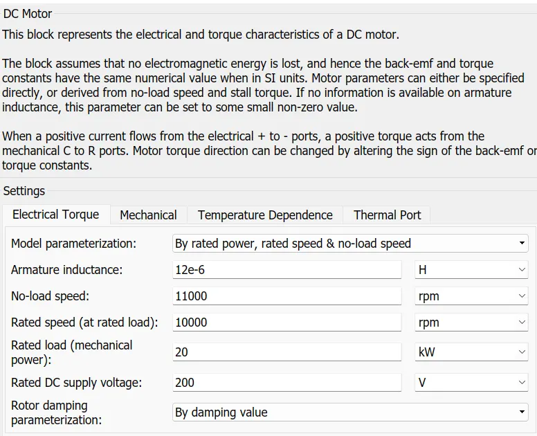
Figure-14 DC motor electrical parameters

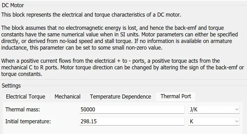
Figure-15 DC motor thermal parameters

Now because we are using a DC motor and the battery supply is also DC, we need a DC/DC converter. In this simulation I have used H-bridge. We need a Pulse width modulation (PWM) signal to operate H-bridge. Also to operate the H- bridge we need to supply the power. Here there are two options External and Internal. We have used Internal power supply. PWM signal amplitude is kept at 5V, which means if the voltage supply is more than 5V, Switch is kept ON.

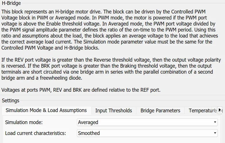
Figure-16 H-bridge Simulation mode

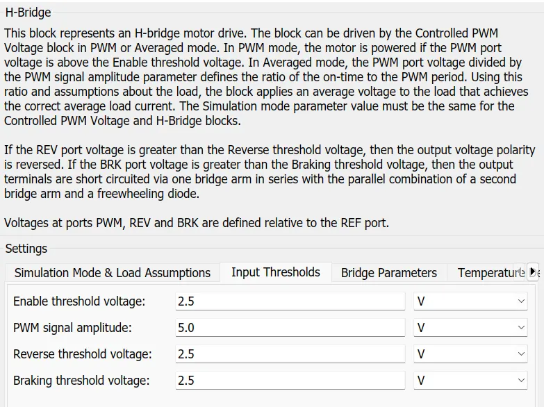
Figure-17 PWM signal amplitude

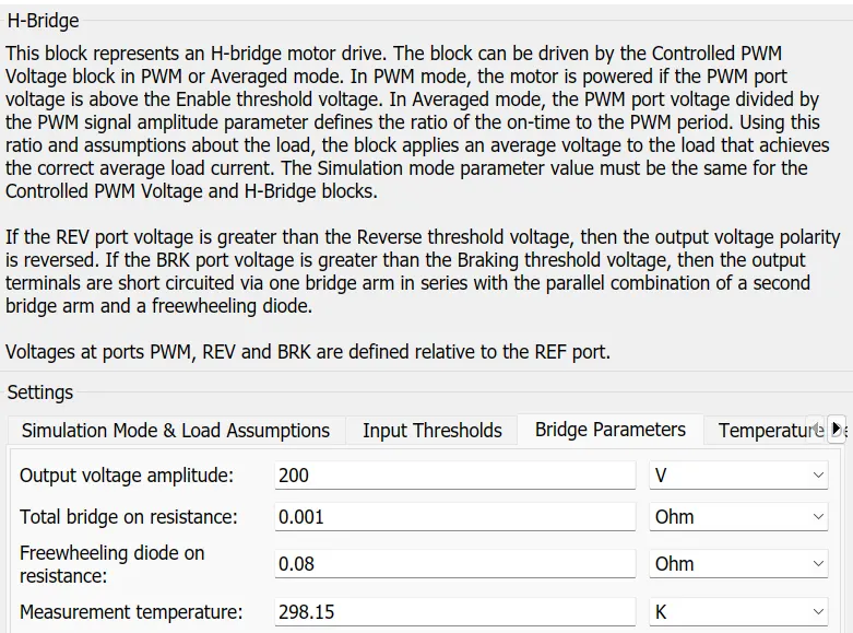
Figure-18 H-bridge output voltage

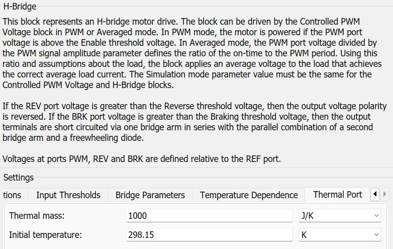
Figure-19 H-bridge thermal mass

These PWM signal are created using PWM controlled voltage. For more time samples, frequency is kept high. Duty cycle input voltage is specified and output voltage is specified as 200V.

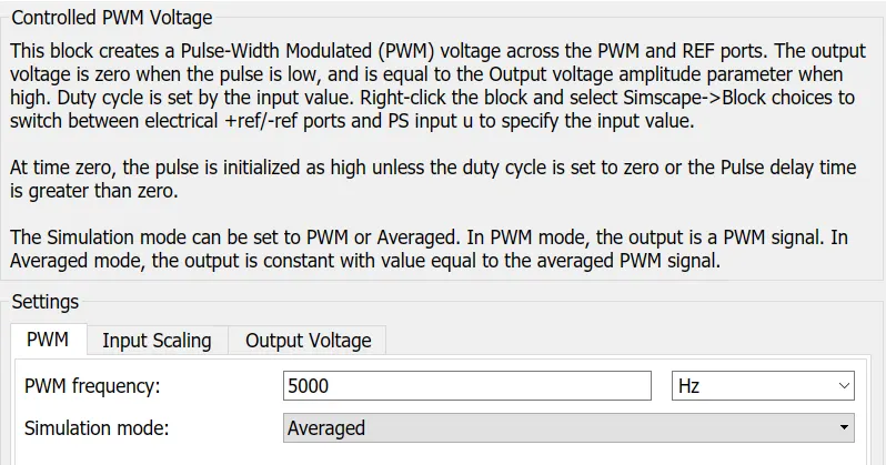
Figure-20 PWM frequency

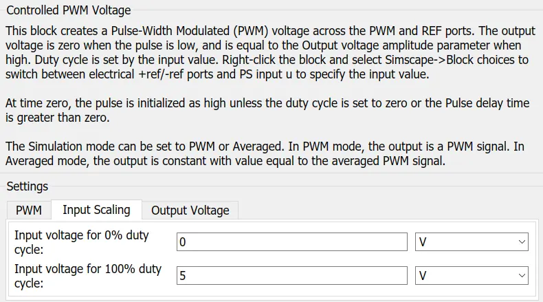
Figure-21 Input voltage for 100% duty cycle

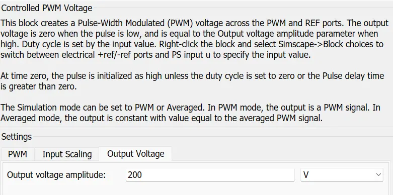
Figure-22 PWM output voltage

Signal to the PWM controlled voltage is coming from the error signal from controller as brake and acceleration command. These command are feeded to PWM controlled voltage through controlled voltage source.

• Battery

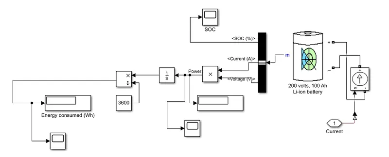
Figure-23 Battery blockset

Blocks used

Controlled current source

Li-ion battery

Bus selector

Integrator

Display and Scope

Divide

Because we are using an internal power supply system in the motor and its controller circuit, we extract the current using a current sensor and give it to the battery using controlled current source. Now the voltage of the battery is decided to be 120V and rated capacity is 120Ah. Battery response time is kept as 5 sec. Sate of charge (SOC), Voltage and Current are extracted using a Bus selector and Energy consumed and Battery state of charge are plotted.

Power = V*I = Energy consumed per unit time

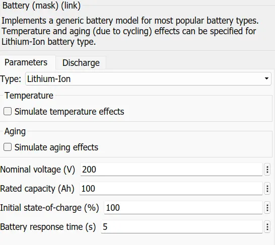
Figure-24 Battery parameters

• Controller or Driver

A proportional–integral–derivative controller (PID controller) is a control loop mechanism employing feedback that is widely used in industrial control systems and a variety of other applications requiring continuously modulated control. A PID controller continuously calculates an error value e(t) as the difference between a desired setpoint and a measured process value and applies a correction based on proportional, integral, and derivative terms (denoted P, I, and D respectively).

Term P is proportional to the current value of the (Setpoint − Process value) error e(t).

Term I accounts for past values of the (Setpoint − Processvalue) error and integrates them over time to produce the I term.

Term D is a best estimate of the future trend of the (Setpoint − Processvalue) error, based on its current rate of change.

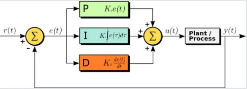
Figure-26 PID basic

General Observations: PID gains

Closed loop response	Rise time	Overshoot	Settling time	Steady state error
Kp (If increased)	Decreases	Increases	Small change	Decreases
Ki (If increased)	Decreases	Increases	Increases	Decreases
Kd (If increased)	Small change	Decreases	Decreases	-

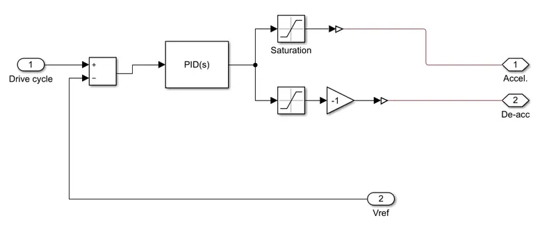
Figure-27 Driver blockset

Referance velocity is the velocity coming from drive cycle. Velocity feedback is taken from the vehicle dynamics. Using a PI controller the error is configured and the value is given to either acceleration or deacceleration command. Now the error is saturated using a saturation block to have separate acceleration and Deacceleration commands. Limits for acceleartion and deacceleration aommand are opposite to each other.

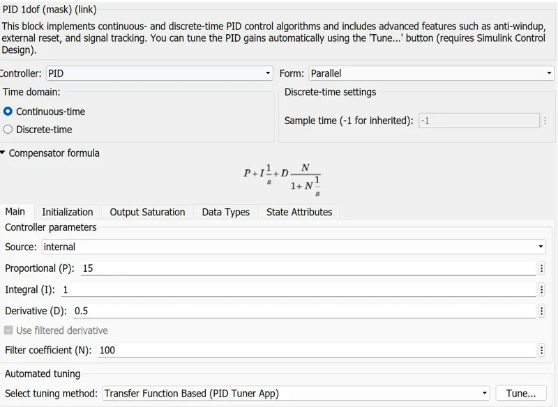
Figure-28 PI values

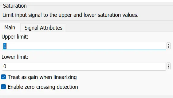
Figure-29 Saturation block

Results:

• Case-1: For FTP75 drive cycle (Kp-15, Ki-1, Kd-0.5)

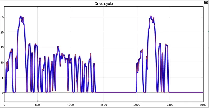
Figure-30 Drive cycle

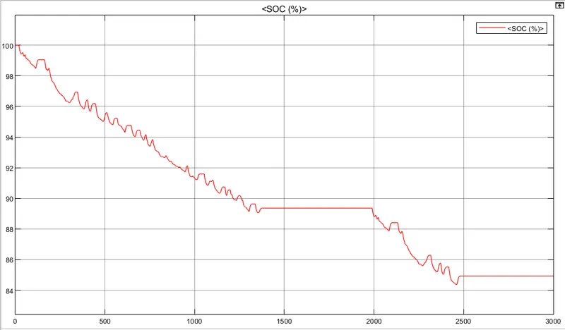
Figure-31 Battery SOC

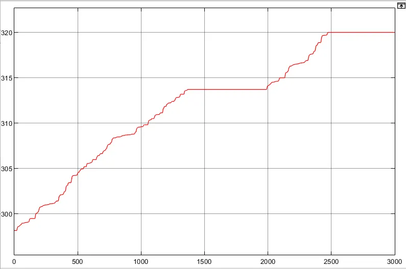
Figure-32 Motor controller temperature

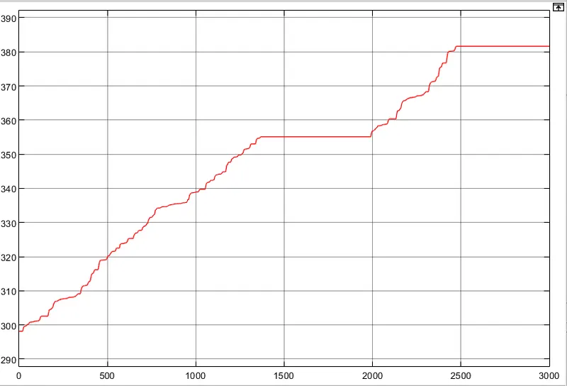
Figure-33 Motor temperature

• Case-2: For Custom made drive cycle (Kp-15, Ki-1, Kd-0.5)

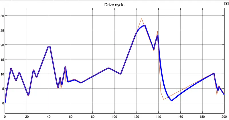
Figure-34 Drive cycle

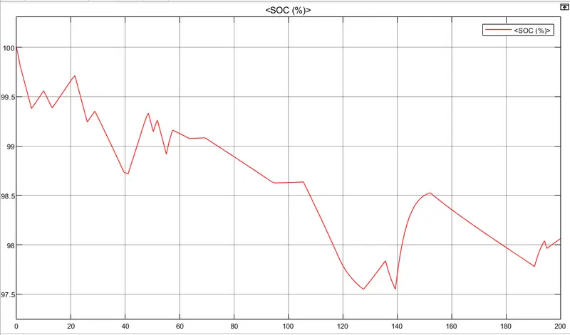
Figure-35 Battery SOC

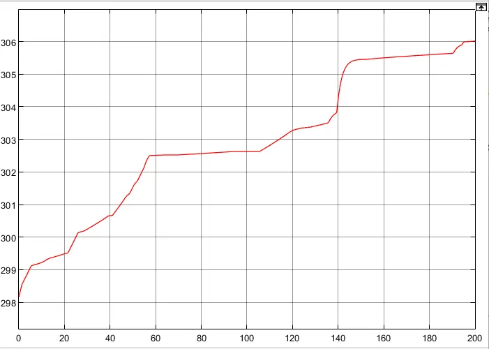
Figure-36 Motor controller temperature

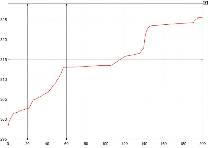
Figure-37 Motor temperature

• Case-3: For constant velocity of 12.5m/s or 45km/hr (Kp-15, Ki-1, Kd-0.5)

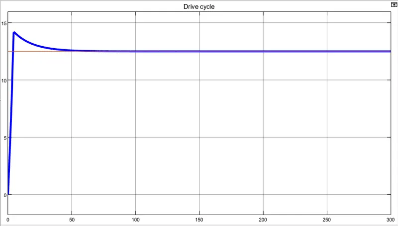
Figure-38 Drive cycle

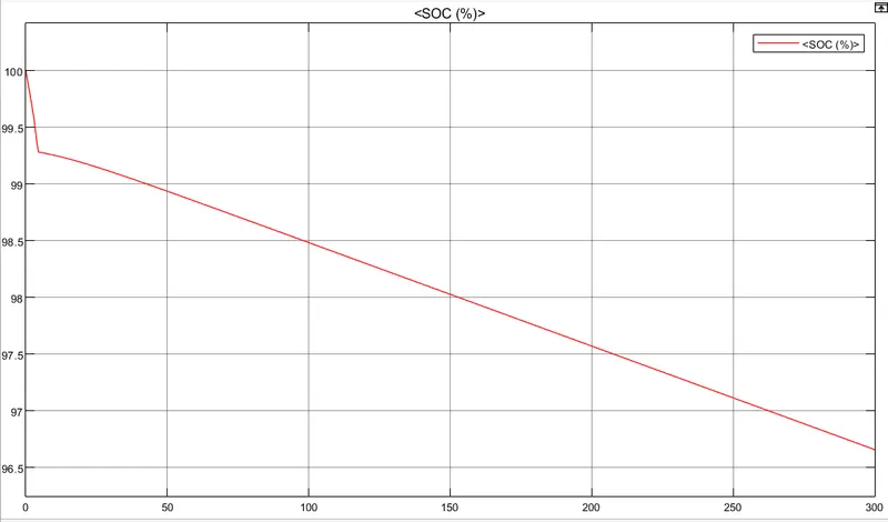
Figure-39 Battery SOC

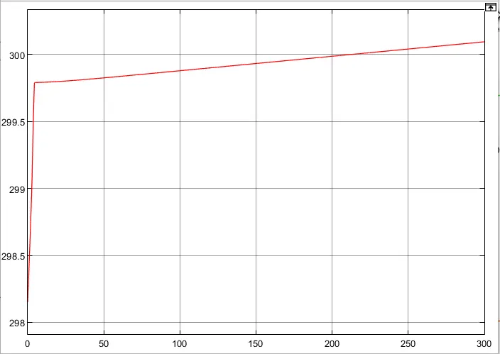
Figure-40 Motor controller temperature

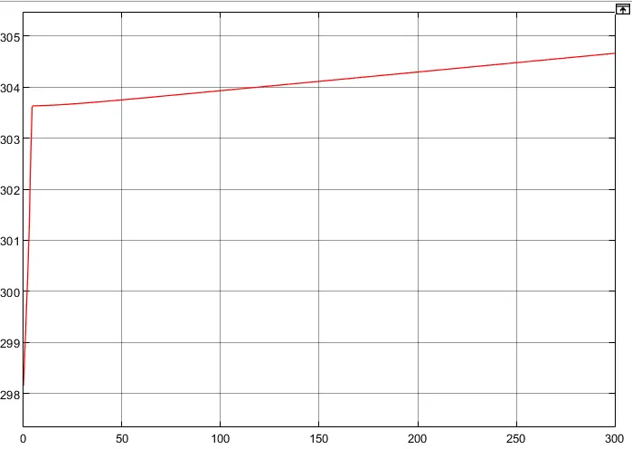
Figure-41 Motor temperature

• Case-4: For constant velocity of 12.5m/s or 45km/hr (Kp-15, Ki-1, Kd-0)

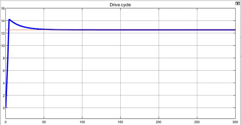
Figure-42 Drive cycle

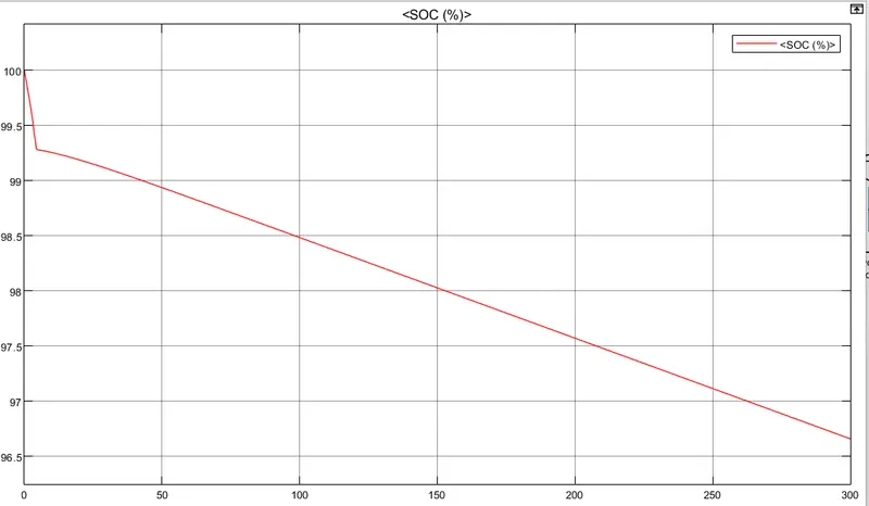
Figure-43 Battery SOC

• Case-5: For constant velocity of 12.5m/s or 45km/hr (Kp-15, Ki-0.5, Kd-10)

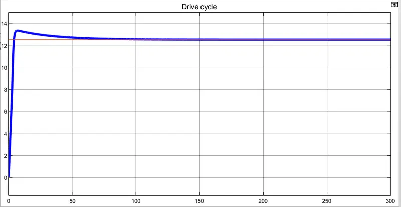
Figure-44 Drive cycle

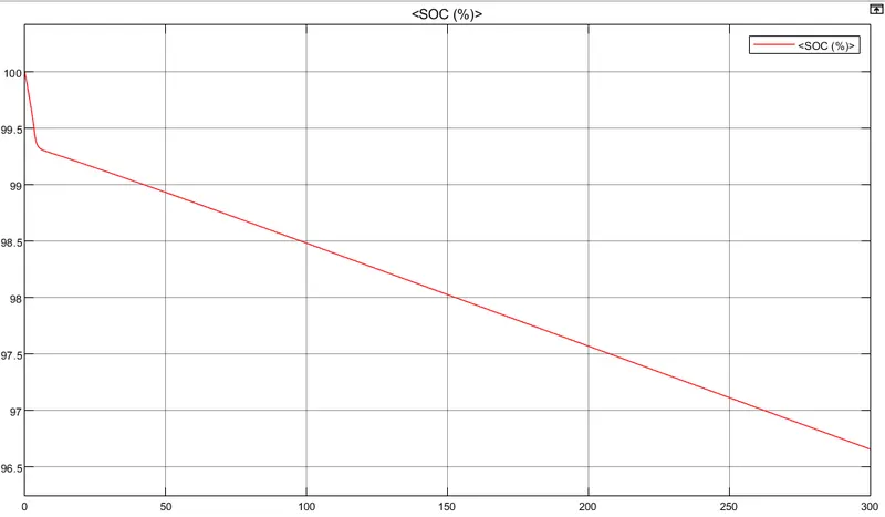
Figure-45 Battery SOC

Table-1

Parameters	FTP75	Custom cycle	Constant 12.5 m/s (Kp-15, Ki-1, Kd-0.5)	Constant 12.5 m/s (Kp-15, Ki-1, Kd-0)	Constant 12.5 m/s (Kp-15, Ki-0.5, Kd-10)
Motor temperature (K)	381.6	325.5	304.7	304.7	303.9
Motor controller temperature (K)	320	306	300.1	300.1	300
Distance covered (Km)	17.78	2.088	3.75	3.75	3.75
Energy consumed (KWh)	2.984	0.32	0.732	0.732	0.734
Battery SOC at the end	85	98.1	96.6	96.6	96.6
Simulation time (s)	3000	200	300	300	300

Conclusion:

• For FTP75 drive cycle, If we run the simulation for 3000 sec, distance covered by the vehicle will be 17.78 Km. After covering 17.78 Km, battery will be discharged by 15 % which means still 85% of the the battery SOC will be present. Motor temperature will be raised to 108.6 deg C (or 381.6K) and the controller temperature will be 47 deg C (or 320 K). Energy consumed will be 2.984 KWh.
• For Custom drive cycle, If we run the simulation for 200 sec, distance covered by the vehicle will be 2.088 Km. After covering 2.088 Km, battery will be discharged by 1.9 % which means still 98.1% of the the battery SOC will be present. Motor temperature will be raised to 52.5 deg C (or 325.5K) and the controller temperature will be 33 deg C (or 306 K). Energy consumed will be 0.32 KWh.
• For constant velocity (12.5 m/s or 45 Km/hr, Kp-15,Ki-1,Kd-0.5) drive cycle, If we run the simulation for 300 sec, distance covered by the vehicle will be 3.75 Km. After covering 3.75 Km, battery will be discharged by 3.4 % which means still 96.6% of the the battery SOC will be present. Motor temperature will be raised to 31.7 deg C (or 304.7K) and the controller temperature will be 27.1 deg C (or 300.1 K). Energy consumed will be 0.732 KWh.
• For constant velocity drive cycle, with decrease in Kd value from 0.5 to 0 (keeping other constants same), no change in the parameters is observed.
• For constant velocity drive cycle, with increase in Kd value from 0.5 to 10 and decreasing Ki from 1 to 0.5 (keeping Kp same), overshoot is decreased. This can be observed from figure(44,42). Also the motor tempearure decreases. Also from figure(42,38), it can be observed that with increase in Kd, settling time decreases.
• Simulink file- https://drive.google.com/file/d/15cR3WewU3SPnHdZjdnk6j4vb6_zIektA/view?usp=sharing